Sediment processes within a reach are directly linked to the capacity of the stream flow to carry eroded soil. The transport capacity of the flow can be calculated from the flow parameters and sediment properties. If the stream can transport more sediment than is contained in the inflow, additional sediment will be eroded from the stream bed and entrained in the flow. However, if the flow in the reach cannot transport the sediment of the inflow, entrained sediment will settle and be deposited to the reach bed. The sediment transport capacity is calculated using the transport potential method. Especially any basin model that uses Muskingum Cunge or kinematic wave routing will need to carefully identify either index flow or index celerity added to each reach element to subdivide the reach into a number of equal length segments (dx) as expressed in the courant condition. Because the volume ratio and linear reservoir sediment routing methods are very sensitive with “dx” may change computed sediment results by numbers of subreach.

The deposition of sediment from the water column to the stream bed requires time. The fall velocity of reach grain size class provides a physical basis for determining how much time is required for sediment in excess of the transport capacity to settle from the water column to the stream bed. The settling velocity is calculated and multiplied by the time interval to determine the settling distance in one time interval. This settling distance is then compared to the flow depth calculated during flow routing in order to determine the fraction of calculated deposition which is actually permitted during a time interval. The approach here is similar to the one used in HEC-RAS.

The erosion of sediment from the stream bed and entraining into the stream flow requires time. Erosion limitation has been observed but the theoretical basis is less clear than for deposition limitation. An empirical rule is used wherein a characteristic flow length necessary for erosion is calculated. Erosion is limited when the length of the reach divided by the flow depth is less than 30. This empirical rule is similar to one used in HEC-RAS.

The reach bed is represented with a two-layer model. The upper layer represents the top of the stream bed which actively interacts with the flow field. This layer responds relatively quickly to changes in flow rate. The lower layer is linked to the upper layer with a simple bed mixing algorithm. The lower layer represents the underlying substrate of the reach. Long-term processes that lead to a reach being either a sediment sink or sediment source within the watershed are represented through the lower layer. The two-layer model is also capable of representing an "armoring" condition, which reduces the rate of erosion as the upper layer coarsens.

As a simplifying assumption, the cross section shape of the channel is fixed. There is no feedback between sediment dynamics and flow routing. A characteristic width and depth of the sediment bed within the reach is used to represent the two-layer model.

Selecting a Sediment Method

The sediment method for a reach is selected on the Component Editor for the reach element (Figure 1). Access the Component Editor by clicking the reach element icon on the "Components" tab of the Watershed Explorer. You can also access the Component Editor by clicking on the element icon in the basin map, if the map is currently open. You can select a sediment method from the list of five available choices. If you choose the None method, the reach will not compute any sediment and all sediment discharges from the element will be zero. Use the selection list to choose the method you wish to use. Each reach may use a different method or several reaches may use the same method.

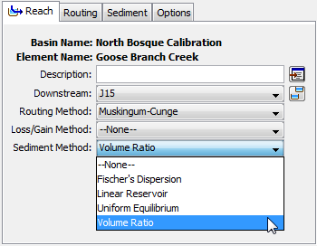
Figure 1. Selecting a channel sediment transport method for a reach element.

The parameters for each sediment method are presented on a separate Component Editor from the reach element editor. The "Sediment" editor is always shown next to the "Routing" editor. The information shown on the sediment editor will depend on which method is currently selected.

Fisher's Dispersion

The Fisher's dispersion method is based on an analysis of the advection and diffusion of sediment within a reach (Fisher et al., 1979). This is the most detailed of the sediment routing methods and requires more data than some of the other available methods. Separate specification of the advection and diffusion parameters for each grain size class permits the large-grained sediments to move slower than the fine-grained sediments. For each time interval, sediment from upstream elements is added to the sediment already in the reach. After erosion or deposition is calculated, the remaining available sediment is translated in the reach by a travel time and attenuated through a diffusion process. The advection and diffusion of the sediment is linked to the velocity of water in the reach which is calculated during the flow routing. The Component Editor is shown in Figure 2.

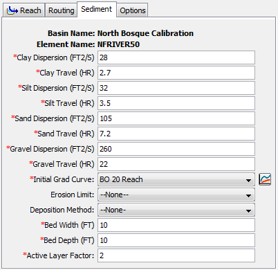
Figure 2. Fisher's dispersion sediment method editor at a reach element.

The dispersion coefficient must be specified for each grain class (clay, silt, sand, gravel). The dispersion coefficient indicates the diffusion of the particles during transit through the reach and is closely connected to channel geometry. The dispersion coefficient can vary over several orders of magnitude and often must be adjusted during calibration. Some guidance is available for estimating the dispersion coefficient, for example, Kashefipour and Falconer (2002). The travel time must also be specified for each grain class (clay, silt, sand, gravel) and is often close to the travel time for water in the reach. When the AGU 20 grain size classification is used, the same dispersion and retention values are used for all subclasses of a grain class.

The initial gradation curve defines the distribution of the bed sediment by grain size at the beginning of the simulation. The same curve is used in both the upper and lower layers of the two-layer bed model. The gradation curve is defined as a diameter-percentage function in the Paired Data Manager. The current functions are shown in the selection list. If there are many different functions available, you may wish to choose a function from the selector accessed with the paired data button next to the selection list. The selector displays the description for each function, making it easier to select the correct one.

Using an erosion limit is optional. When the erosion limit is deactivated, erosion is limited only by the transport capacity of the flow. When the erosion limit is activated, actual erosion is reduced when the ratio of reach length to flow depth is less than 30. The erosion limit is usually encountered only in very short reaches.

Using a deposition limit is optional. When the deposition limit is deactivated, sediment in excess of the transport capacity is deposited completely. When the deposition limit is activated, sediment is limited by the flow depth calculated during flow routing and the fall velocity of each grain size. The fall velocity is computed using the method selected with the basin model properties. Using a deposition limit requires the specification of the water temperature in the reach. You may specify a fixed temperature or select a temperature time-series gage. Temperature gages must be created in the Time-Series Data Manager before they can be used for the sediment method.

The width of the sediment bed must be specified. The width should be typical of the reach and is used in computing the volume of the upper and lower layers of the bed model. The depth of the bed must also be specified. The depth should be typical of the total depth of the upper and lower layers of the bed, representing the maximum depth of mixing over very long time periods.

The active layer factor is used to calculate the depth of the upper layer of the bed model. At each time interval, the upper layer depth is computed as the d₉₀ of the sediment in the upper layer, multiplied by the active layer factor.

Linear Reservoir

The linear reservoir method uses a simple linear reservoir to route each grain size through the reach. For each time interval, available sediment is calculated from the upstream sediment and local erosion or deposition. The available sediment in each grain size class is routed through a linear reservoir independently of the hydrologic routing of the flow. This allows sediment of different grain sizes to move at different speeds through the reach. Calibration with observed data significantly improves the results. The Component Editor is shown in Figure 3.

The retention parameter is equivalent to the storage coefficient in the linear reservoir used to route the sediment through the reach. The routing is performed separately for clay, silt, sand, and gravel. When the AGU 20 grain size classification is used, the same retention is used for all subclasses of each class. The value of the retention parameter is analogous to the median length of time for each sediment class to transit the reach. It may change for each sediment size class but is often close to the travel time for water in the reach.

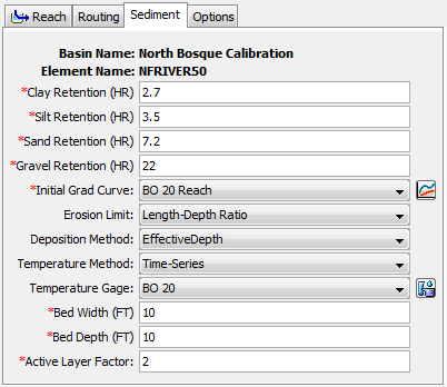
Figure 3. Linear reservoir sediment method editor at a reach element.

The initial gradation curve defines the distribution of the bed sediment by grain size at the beginning of the simulation. The same curve is used in both the upper and lower layers of the two-layer bed model. The gradation curve is defined as a diameter-percentage function in the Paired Data Manager. The current functions are shown in the selection list. If there are many different functions available, you may wish to choose a function from the selector accessed with the paired data button next to the selection list. The selector displays the description for each function, making it easier to select the correct one.

Using an erosion limit is optional. When the erosion limit is deactivated, erosion is limited only by the transport capacity of the flow. When the erosion limit is activated, actual erosion is reduced when the ratio of reach length to flow depth is less than 30. The erosion limit is usually encountered only in very short reaches.

Using a deposition limit is optional. When the deposition limit is deactivated, sediment in excess of the transport capacity is deposited completely. When the deposition limit is activated, sediment is limited by the flow depth calculated during flow routing and the fall velocity of each grain size. The fall velocity is computed using the method selected with the basin model properties. Using a deposition limit requires the specification of the water temperature in the reach. You may specify a fixed temperature or select a temperature time-series gage. Temperature gages must be created in the Time-Series Data Manager before they can be used for the sediment method.

The width of the sediment bed must be specified. The width should be typical of the reach and is used in computing the volume of the upper and lower layers of the bed model. The depth of the bed must also be specified. The depth should be typical of the total depth of the upper and lower layers of the bed, representing the maximum depth of mixing over very long time periods.

The active layer factor is used to calculate the depth of the upper layer of the bed model. At each time interval, the upper layer depth is computed as the d₉₀ of the sediment in the upper layer, multiplied by the active layer factor.

Uniform Equilibrium

The uniform equilibrium method assumes that sediment is translated instantaneously through the reach. It is the simplest method because it does not compute any temporal lag for the sediment passing through the reach. Sediment enters the reach from upstream elements. The transport capacity for each grain size is calculated to determine the deposition or erosion state. The available sediment is computed subject to the limitations on deposition and erosion. The available sediment is then passed out of the reach regardless of the velocity determined during flow routing. The Component Editor is shown in Figure 4.

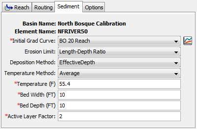
Figure 4. Uniform equilibrium sediment method editor at a reach element.

The initial gradation curve defines the distribution of the bed sediment by grain size at the beginning of the simulation. The same curve is used in both the upper and lower layers of the two-layer bed model. The gradation curve is defined as a diameter-percentage function in the Paired Data Manager. The current functions are shown in the selection list. If there are many different functions available, you may wish to choose a function from the selector accessed with the paired data button next to the selection list. The selector displays the description for each function, making it easier to select the correct one.

Using an erosion limit is optional. When the erosion limit is deactivated, erosion is limited only by the transport capacity of the flow. When the erosion limit is activated, actual erosion is reduced when the ratio of reach length to flow depth is less than 30. The erosion limit is usually encountered only in very short reaches.

Using a deposition limit is optional. When the deposition limit is deactivated, sediment in excess of the transport capacity is deposited completely. When the deposition limit is activated, sediment is limited by the flow depth calculated during flow routing and the fall velocity of each grain size. The fall velocity is computed using the method selected with the basin model properties. Using a deposition limit requires the specification of the water temperature in the reach. You may specify a fixed temperature or select a temperature time-series gage. Temperature gages must be created in the Time-Series Data Manager before they can be used for the sediment method.

The width of the sediment bed must be specified. The width should be typical of the reach and is used in computing the volume of the upper and lower layers of the bed model. The depth of the bed must also be specified. The depth should be typical of the total depth of the upper and lower layers of the bed, representing the maximum depth of mixing over very long time periods.

The active layer factor is used to calculate the depth of the upper layer of the bed model. At each time interval, the upper layer depth is computed as the d₉₀ of the sediment in the upper layer, multiplied by the active layer factor.

Volume Ratio

The volume ratio method links the transport of sediment to the transport of flow in the reach using a conceptual approach. For each time interval, sediment from upstream elements is added to the sediment already in the reach. The deposition or erosion of sediment is calculated for each grain size to determine the available sediment for routing. The proportion of available sediment that leaves the reach in each time interval is assumed equal to the proportion of stream flow that leaves the reach during that same interval. This means that the all grain sizes are transported through the reach at the same rate, even though erosion and deposition are determined separately for each grain size. This assumption essentially limits the advection velocity of the sediment to the bulk water velocity. Therefore, this method is a higher fidelity option than the Equilibrium method (without requiring much more data) but less precise than the other available methods which require substantially more data. This method is very similar to the approach used in the Soil and Water Assessment Tool model (Gassman, 2007). The Component Editor is shown in Figure 5.

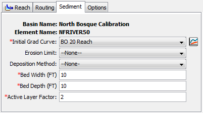
Figure 5. Volume ratio sediment method editor at a reach element.

The initial gradation curve defines the distribution of the bed sediment by grain size at the beginning of the simulation. The same curve is used in both the upper and lower layers of the two-layer bed model. The gradation curve is defined as a diameter-percentage function in the Paired Data Manager. The current functions are shown in the selection list. If there are many different functions available, you may wish to choose a function from the selector accessed with the paired data button next to the selection list. The selector displays the description for each function, making it easier to select the correct one.

Using an erosion limit is optional. When the erosion limit is deactivated, erosion is limited only by the transport capacity of the flow. When the erosion limit is activated, actual erosion is reduced when the ratio of reach length to flow depth is less than 30. The erosion limit is usually encountered only in very short reaches.

Using a deposition limit is optional. When the deposition limit is deactivated, sediment in excess of the transport capacity is deposited completely. When the deposition limit is activated, sediment is limited by the flow depth calculated during flow routing and the fall velocity of each grain size. The fall velocity is computed using the method selected with the basin model properties. Using a deposition limit requires the specification of the water temperature in the reach. You may specify a fixed temperature or select a temperature time-series gage. Temperature gages must be created in the Time-Series Data Manager before they can be used for the sediment method.

The width of the sediment bed must be specified. The width should be typical of the reach and is used in computing the volume of the upper and lower layers of the bed model. The depth of the bed must also be specified. The depth should be typical of the total depth of the upper and lower layers of the bed, representing the maximum depth of mixing over very long time periods.

The active layer factor is used to calculate the depth of the upper layer of the bed model. At each time interval, the upper layer depth is computed as the d₉₀ of the sediment in the upper layer, multiplied by the active layer factor.