In addition to viewing results for the currently selected simulation run, it is also possible to view results for other runs that are not the current selection. Those other runs are also tracked in the same way as the current run to make sure data has not changed and results do not need to be recomputed. Results for other simulation runs are accessed through the Watershed Explorer, on the "Results" tab.

To begin viewing results, go to the "Results" tab of the Watershed Explorer and click on the desired simulation run icon. If necessary, click on the "Simulation Runs" folder to expand it and view the simulation runs in the project. The simulation run icon will be disabled if results have not been computed. If any result is open at the time data changes, the affected results will be automatically updated when the simulation run is recomputed.

Global Summary Table

The global summary table can be accessed by clicking on the "Global Summary" node in the Watershed Explorer (Figure 1). The global summary table will open. It is exactly the same table that can be viewed for the current simulation run. The table includes one row for each element in the basin model and columns for element name, drainage area, peak flow, time of peak flow, and total outflow volume.

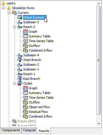
Figure 1. Accessing simulation run results from the Watershed Explorer.

Individual Elements

Each element in the basin model is shown in the Watershed Explorer under the simulation run node. These elements are listed in hydrologic order below the global summary table. The results for each element are accessed by clicking on its node. The first item listed for each element is the graph; click on the "Graph" node to view the result (Figure 1). It is exactly the same graph that can be viewed for the current simulation run. The information included in the graph varies by element type but always includes outflow. Optional items such as observed flow, computed stage, and observed stage are also included. Similarly, the summary table and time-series table can also be accessed by clicking on the "Summary Table" or "Time-Series Table" node, respectively.

Element Time-Series Preview Graph

All of the time-series data computed by an individual element are available for viewing. The time-series data are listed under each element node in the Watershed Explorer. The first node under each element is the graph, followed by the summary table and time-series table. The remaining nodes for each element represent the different time-series data available at that element. Click on a time-series node to preview the data in the Component Editor. You may select multiple time-series data by holding the shift or control key while using the mouse to click on additional nodes (Figure 2). The selected time-series may come from different elements in the same simulation run, the same element in different runs, or different elements in different runs. The selected time-series data will automatically be partitioned into groups by data type.

Time-Series Tables and Graphs

Preview graphs of selected time-series data can be opened as graphs or time-series tables within the Desktop area. Begin by selecting the time-series you wish to include in the graph or table. Once you have selected the desired time-series, you can press the graph or time-series table buttons on the toolbar. The chosen time-series will be graphed or tabulated (Figure 3).

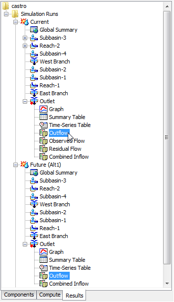
Figure 2. Selecting computed outflow from the same element in two different simulation runs. Other types of time-series data could also be selected.

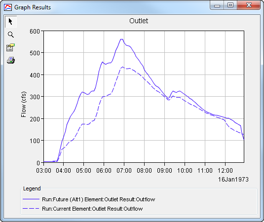
Figure 3. Custom graph created by selecting multiple time-series results for a preview and then pressing the graph button on the toolbar.

After you have opened a time-series table or graph, you may add additional time-series results. Position the mouse over the time-series result in the Watershed Explorer that you wish to add to the graph or table. Press and hold the left mouse button and then drag the mouse over the top of the graph or table where you want the result to be added. The mouse cursor will change to indicate which tables and graphs can accept the additional time-series. Release the mouse button while it is over the desired table or graph and it will be automatically updated to show the additional time-series results.

Changing Graph Properties

All of the graphs that can be accessed open with default properties for line color, line style, data symbols, etc. These default properties have been selected to be appropriate for most situations. However, it is possible to customize the properties in a graph. To change the properties, first click on the graph to select it. Next go to the Results menu and select the Graph Properties… command. An editor (Figure 4) will open that can be used to change the properties of the selected graph. The properties for each time-series curve can be changed. It is also possible to change the properties for the axis, title, gridlines, patterns, and legend.

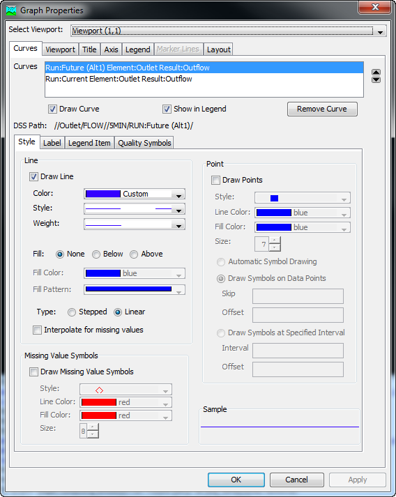
Figure 4. Editing the drawing properties for an element graph.