Download PDF
Download page Viewing Spatial Results.
Viewing Spatial Results
The Spatial Results toolbar provides options to visualize results for basin models that have been created using GIS features (georeferenced elements). Spatial results must be turned on within the simulation run's Component Editor. Spatial results should be turned on after preliminary calibration has been completed. Use of spatial results can assist in the calibration process and provide additional information about the simulation. If you make edits to the basin geometry, edit model parameters, or change the simulation configuration, the spatial results will be automatically re-computed during the simulation.
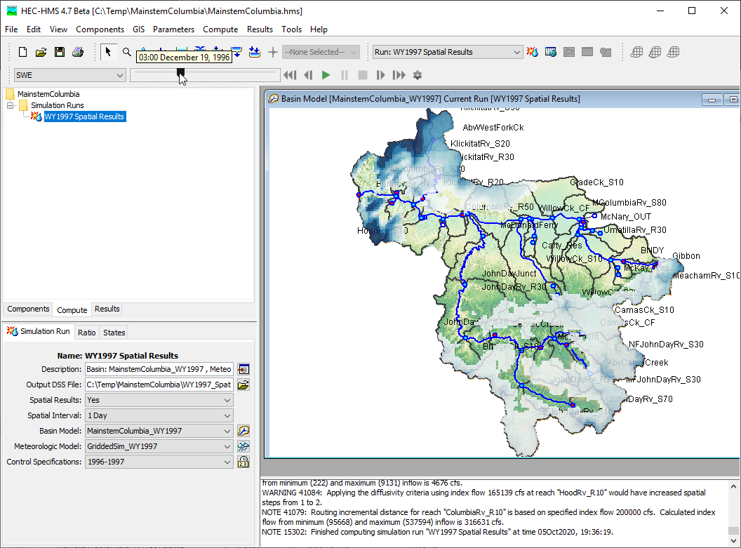
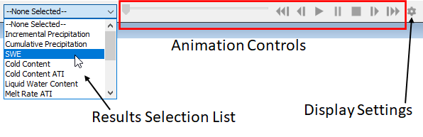
The following figure shows the Spatial Results toolbar along with Snow Water Equivalent (SWE) results displayed on top of the basin model. The Spatial Results toolbar includes options for selecting output results, an animation toolbar, buttons for controlling the animation, and a display settings button that opens an editor with options for animation, symbology, and display setting.
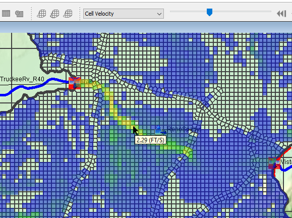
When a valid spatial result is selected, a tool tip containing the value and units for the specific time step and grid cell over which the mouse is hovered will be displayed, as shown in the following figure.
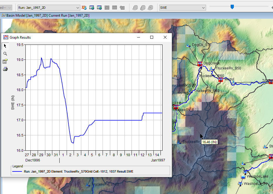
When a valid spatial result is selected, the right click | Plot Spatial Results option is available for tabulating the results for the specific grid cell which was clicked, as shown in the following figure.
Requirements for Spatial Results
A georeferenced basin model (subbasin elements must be georeferenced) is required to utilize spatial results. A georeferenced basin model can be created using the GIS tools to delineate elements from a terrain model. Another option to georeference a basin model is to use the Georeference Existing Elements or Import Georeferenced Elements tools from the GIS menu. These two tools use geographic information in shapefiles to georeference subbasin elements.
Spatial results can be visualized at the subbasin level, spatially averaged for the subbasin, or across the model domain using the discretization method chosen for the subbasin elements (structured discretization or unstructured discretization). Spatial results will be displayed at the grid or mesh level when the transform method is either ModClark or 2D Diffusion Wave and the structured, unstructured, and File-Specified *.sqlite, *.HDF5, and *.HDF discretization methods are selected. Gridded spatial results cannot be visualized for subbasin elements using the ModClark file option (under the File-Specified discretization method). Instead, results will be displayed as a subbasin average value when the *.mod file option is used for the File-Specified discretization method. Spatial results will be displayed at the subbasin level when transform methods other than the ModClark or 2D Diffusion Wave transform are used.
Activate Spatial Results
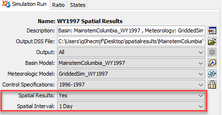
Spatial results can be displayed for both simulation runs and forecast alternatives. Spatial results must be activated in the simulation run's Component Editor, as shown below. You can also set the time interval for spatial results. The simulation time-step is used as the default interval. Spatial results are saved to an HDF5 file within the project's "results" directory; results are saved to an *.H5 file. Turning on spatial results will add additional time to the simulation due to additional output being generated and saved to disk. The additional time can be up to 1/3 of the simulation time without spatial results activated.
The very first time an output result is selected in the Spatial Results toolbar, the program will process the simulation HDF5 and build animation tiles for display. A message will pop up the very first time the output HDF file is processed indicating animation tiles are being created. The time it takes to build the animation tiles can be large for larger model domains; however, the processing is only required the very first time spatial results are displayed. The display time for subsequent simulations will be much quicker because animation information already exists.
Spatial Results Toolbar
As shown in the figure below, the Spatial Results toolbar is configured to 1) select an output result to visualize, 2) control the animation, and 3) edit the display and animation properties. Results that can be animated include meteorologic results, snow modeling results, and precipitation excess and loss. Hydraulic depth, water surface elevation, and cell velocity can be displayed for subbasins that use the 2D Diffusion Wave transform method. A full list of spatial variables is provided below (some results are only available when running the program in debug mode):
| Variable | Process | Method |
|---|---|---|
| Incremental Precipitation | Precipitation | All Precipitation Methods |
| Cumulative Precipitation | Precipitation | All Precipitation Methods |
| SWE (Snow Water Equivalent) | Snowmelt | All Snowmelt Methods |
| Albedo | Snowmelt | Energy Balance |
| ATI (Antecedent Temperature Index) | Snowmelt | Temperature Index |
| Cold Content | Snowmelt | Temperature Index |
| Cold Content ATI | Snowmelt | Temperature Index |
| Heat Deficit | Snowmelt | RTI/Hybrid |
| Liquid Water Content | Snowmelt | All Snowmelt Methods |
| Melt Rate ATI | Snowmelt | Temperature Index |
| Pack Energy | Snowmelt | Energy Balance |
| Pack Temperature | Snowmelt | Energy Balance |
| Snow Depth | Snowmelt | RTI/Hybrid and Energy Balance |
| Surface Temperature | Snowmelt | Energy Balance |
| Incremental Loss | Loss | All Loss Methods |
| Cumulative Loss | Loss | All Loss Methods |
| Incremental Excess | Loss | All Loss Methods |
| Cumulative Excess | Loss | All Loss Methods |
| Water Surface Elevation | Transform | 2D Diffusion Wave |
| Hydraulic Depth | Transform | 2D Diffusion Wave |
| Cell Velocity | Transform | 2D Diffusion Wave |
| Bed Change (Total) | Sediment Transport | 2D Sediment |
| Bed Change - Clay | Sediment Transport | 2D Sediment |
| Bed Change - Silt | Sediment Transport | 2D Sediment |
| Bed Change - Sand | Sediment Transport | 2D Sediment |
| Bed Change - Gravel | Sediment Transport | 2D Sediment |
| Sediment Concentration (Total) | Sediment Transport | 2D Sediment |
| Sediment Concentration - Clay | Sediment Transport | 2D Sediment |
| Sediment Concentration - Silt | Sediment Transport | 2D Sediment |
| Sediment Concentration - Sand | Sediment Transport | 2D Sediment |
| Sediment Concentration - Gravel | Sediment Transport | 2D Sediment |
The animation can be controlled through the animation control slider bar and buttons. The slider bar can be manually dragged right or left to advance or reverse results. The animation control buttons include a button to go to the beginning of the animation, move forward one time interval, pause the animation, reverse the animation one time interval, and go to the end of the animation.
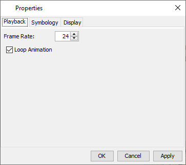
The Display Settings editor can be opened by clicking the gear icon located on the right side of the Spatial Properties toolbar. The figure below shows the Playback tab in the Display Settings editor. You can change the Frame Rate to control the speed of the animation. There is check box to control whether the animation is looped or not.
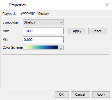
The figure below shows the Symbology tab. When the Stretch Symbology option is selected, you can edit the Max and Min values and the Color Scheme.
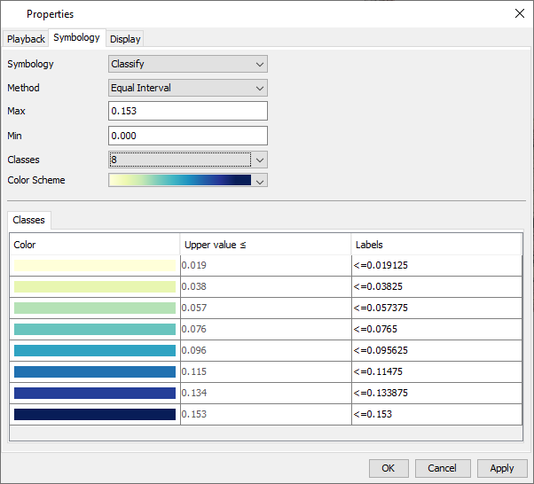
The figure below shows how the Symbology editor is configured when the Classify Symbology option is selected. There are three methods to choose from to subdivide classes, Natural Breaks (Jenks), Equal Interval, and Manual. You can overwrite the Max and Min values when the Equal Interval option is selected. You can edit the Upper values in the Classes table when the Manual method is selected. The number of Classes can only be edited when the Natural Breaks (Jenks) or Equal Interval methods are chosen. You can edit the Color Scheme by choosing a palette from the drop down list, you can also edit individual colors by clicking on them in the Classes table. Finally, Labels can be manually edited if needed.
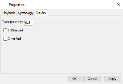
The figure below shows the Display tab. You can control the Transparency setting, and whether to apply hillshading or to invert the color ramp.
The Apply button must be pressed after edits are made to the display settings, then press the Close button to close the editor.