Evapotranspiration is the the combination of evaporation from the ground surface and transpiration by vegetation. It includes both evaporation of free water from the surface of vegetation and the land surface. It also includes transpiration which is the process of vegetation extracting it from the soil through the plant root system. Whether by evaporation or transpiration, water is returned from the land surface or subsurface to the atmosphere. Even though evaporation and transpiration are taken together, transpiration is responsible for the movement of much more water than evaporation. Combined evapotranspiration is often responsible for returning 50 or even 60% of precipitation back to the atmosphere. The theoretical evapotranspiration, also called the potential evapotranspiration, serves as the upper limit for what can happen on the land surface based on atmospheric conditions. In all cases, the meteorologic model is computing the potential evapotranspiration and subbasins will calculate actual evapotranspiration based on soil water limitations.

The evapotranspiration method included in the meteorologic model is only necessary when using continuous simulation loss rate methods in subbasins: deficit constant, gridded deficit constant, soil moisture accounting, and gridded soil moisture accounting. If a continuous simulation loss rate method is used and no evapotranspiration is specified in the meteorologic model, then zero potential evapotranspiration is used in the subbasins. The options for evapotranspiration include a physically-based energy balance model (Penman Monteith), a simplified physically-based model (Priestley Taylor), the Hargreaves and Hamon temperature only methods, and a simple monthly average approach. A specified method is also included so that evapotranspiration can be calculated external to the program and imported. Each option produces the potential evapotranspiration rate over the land surface where it can be used in the subbasin element to compute evaporation from the canopy and surface, and transpiration from the soil. More detail about each method is provided in the following sections.

Annual Evapotranspiration

The annual evapotranspiration method is designed to work with a maximum daily rate combined with an optional pattern of variation throughout the year. Specifying only a daily rate can produce good results for simulations lasting days to weeks if evapotranspiration is fairly consistent each day. The optional pattern can be used to adjust the applied evapotranspiration rate during simulations lasting weeks to years.

The annual evapotranspiration method includes a Component Editor with parameter data for all subbasins in the meteorologic model. The Watershed Explorer provides access to the evapotranspiration component editor using a picture of a water pan.

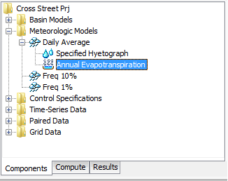
Figure 1. A meteorologic model using the annual evapotranspiration method with a single component editor for all subbasins.

The Component Editor for all subbasins in the meteorologic model includes the daily rate and optional pattern for each subbasin. When the optional percentage pattern is not used, the value entered for the daily rate should generally be the average daily potential evapotranspiration rate over the duration of the simulation. When a pattern will be added, the value entered for the daily rate should generally be the largest potential evapotranspiration for any day occurring during the simulation.

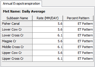
Figure 2. Entering rates and selecting a percent pattern for each subbasin.

The optional pattern is specified as a percent pattern in the paired data manager. The evapotranspiration for each day of the simulation is computed by multiplying the entered rate by the percentage interpolated from the percent pattern. The available percent patterns are shown in the selection list. If there are many different patterns available, you may wish to choose a pattern from the selector accessed with the paired data button next to the selection list. The selector displays the description for each percent pattern, making it easier to select the correct one.

Gridded Hamon

The gridded Hamon method is the same as the regular Hamon method (described in a later section) except that the Hamon equations are applied to each grid cell using separate boundary conditions instead of area-averaged values over the whole subbasin. The gridded Hamon method requires no gridded shortwave radiation method or gridded longwave radiation method in the meteorologic model.

The gridded Hamon method includes a Component Editor with parameter data for all subbasins in the meteorologic model. The Watershed Explorer provides access to the evapotranspiration component editor using a picture of a water pan (Figure 3).

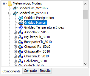
Figure 3. A meteorologic model using the gridded Hamon evapotranspiration method with a component editor for all subbasins.

The Component Editor requires a temperature gridset be selected for all subbasins. (Figure 4). The current gridset is shown in the selection list. If there are many different gridsets available, you may wish to choose a gridset from the selector accessed with the grid button next to the selection list.

The Component Editor requires a Hamon coefficient be selected for all subbasins (Figure 4). A default coefficient of 0.0065 inches per gram per meter cubed is provided; this is equivalent to 0.1651 millimeters per gram per meter cubed. The units inches per gram per meter cubed are implicit in the Hamon (1963) formulation where the coefficient is presented as a constant: 0.0065. The coefficient can be adjusted by the user in the component editor.

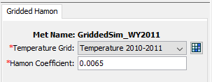
Figure 4. Component editor for the gridded Hamon evapotranspiration method.

Gridded Hargreaves

The gridded Hargreaves method is the same as the regular Hargreaves method (described in a later section) except that the Hargreaves equations are applied to each grid cell using separate boundary conditions instead of area-averaged values over the whole subbasin. Shortwave radiation is required in the Hargreaves method so a gridded shortwave radiation method should also be selected in the meteorologic model.

The gridded Hargreaves method includes a Component Editor with parameter data for all subbasins in the meteorologic model. The Watershed Explorer provides access to the evapotranspiration component editor using a picture of a water pan (Figure 5).

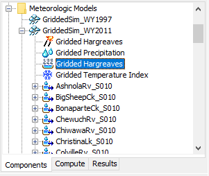
Figure 5. A meteorologic model using the gridded Hargreaves evapotranspiration method with a component editor for all subbasins.

The Component Editor requires a temperature gridset be selected for all subbasins. (Figure 6). The current gridset is shown in the selection list. If there are many different gridsets available, you may wish to choose a gridset from the selector accessed with the grid button next to the selection list.

The Component Editor for all subbasins includes a Hargreaves evapotranspiration coefficient (Figure 6). A default coefficient of 0.0075 per degree Fahrenheit is provided; this is equivalent to 0.0135 per degree Celsuis. If the gridded Hargreaves evapotranspiration method is combined with the gridded Hargreaves shortwave radiation method, the resulting default coefficient is 0.0023 per degree Celsius raised to the 3/2 power. This is equivalent to the form presented by Hargreaves and Allen (2003), Eq. 8.

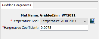
Figure 6. Component editor for the gridded Hargreaves evapotranspiration method.

Gridded Penman Monteith

The gridded Penman Monteith method is designed to work with the gridded ModClark transform method. It is the same as the regular Penman Monteith method (described in a later section) except that the Penman Monteith equations are applied to each grid cell using separate boundary conditions instead of area-averaged values over the whole subbasin. Shortwave and longwave radiation are inputs to the Penman Monteith method so both a gridded shortwave radiation method and a gridded longwave radiation method should also be selected in the meteorologic model.

The gridded Penman Monteith method includes a Component Editor with parameter data for all subbasins in the meteorologic model. The Watershed Explorer provides access to the evapotranspiration component editor using a picture of a water pan (Figure 7).

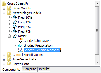
Figure 7. A meteorologic model using the gridded Penman Monteith evapotranspiration method with a component editor for all subbasins.

The Component Editor for all subbasins in the meteorologic model includes parameter grids for the atmospheric variables required in the Penman Monteith equations (Figure 8). A temperature gridset must be selected for all subbasins. The current gridsets are shown in the selection list. If there are many different gridsets available, you may wish to choose a gridset from the selector accessed with the grid button next to the selection list. The selector displays the description for each gridset, making it easier to select the correct one. A gridset is also required for windspeed. Actual vapor pressure deficit can be calculated using the dew point temperature, relative humidity, or daily minimum temperature. The daily minimum temperature option should be used when relative humidity or dewpoint data are not available; the daily minimum temperature option assumes the dewpoint temperature is equal to the daily minimum temperature. The water vapor method will require a relative humidity, dew point temperature, or air temperature gridset depending on the vapor pressure type selected.

A reference albedo is required for computing the energy balance at the ground surface. The same value is applied to all grid cells in all subbasins. A default value of 0.23 is provided.

Figure 8. Component editor for the gridded Penman Monteith evapotranspiration method.

Gridded Priestley Taylor

The gridded Priestley Taylor method is designed to work with the gridded ModClark transform method. It is the same as the regular Priestley Taylor method (described in a later section) except the Priestley Taylor equations are applied to each grid cell using separate boundary conditions instead of area-averaged values over the whole subbasin. Net shortwave radiation is an input to the Priestley Taylor method so a gridded shortwave radiation method should also be selected in the meteorologic model.

The gridded Priestley Taylor method includes a Component Editor with parameter data for all subbasins in the meteorologic model. The Watershed Explorer provides access to the evapotranspiration component editor using a picture of a water pan (Figure 9).

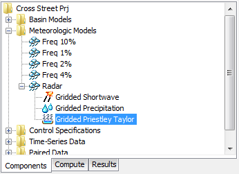
Figure 9. A meteorologic model using the gridded Priestley Taylor evapotranspiration method with a component editor for all subbasins.

The Component Editor for all subbasins in the meteorologic model includes a dryness coefficient which must be entered for all subbasins (Figure 10). The same coefficient is applied to all grid cells in all subbasins. The coefficient is used to make small corrections based on soil moisture state. A coefficient should be specified that represents typical soil water conditions during the simulation. A value of 1.2 can be used in humid conditions while a value of 1.3 represents an arid environment.

A temperature gridset must be selected for all subbasins. The current gridsets are shown in the selection list. If there are many different gridsets available, you may wish to choose a gridset from the selector accessed with the grid button next to the selection list. The selector displays the description for each gridset, making it easier to select the correct one.

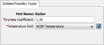
Figure 10. Component editor for the gridded Priestley Taylor evapotranspiration method.

Hamon

The Hamon method (Hamon, 1963) is based on an empirical relationship where saturated water vapor concentration, at the mean daily air temperature, adjusted by a day length factor, is proportional to potential evapotranspiration. The day length factor accounts for plant response, duration of turbulence, and net radiation. Daily average temperature is the only data requirement. The method has proven effective for estimating potential evapotranspiration in data-limited situations. The method calculates daily potential evaptranspriation given daily average temperature. For simulation time steps less than one day, potential evapotranspiration is redistributed for each time step based on a sinusoidal distribution between sunrise and sunset.

The Hamon method includes a Component Editor with parameter data for each individual subbasin in the meteorologic model. The Watershed Explorer provides access to the evapotranspiration component editor using a picture of a water pan (Figure 11). An air temperature gage must be selected in the atmospheric variables Component Editor for each subbasin. To open the atmospheric variables Component Editor, click on a subbasin node in the Watershed Explorer.

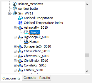
Figure 11. A meteorologic model using the Hamon evapotranspiration method with a component editor for each individual subbasin.

The Component Editor for each subbasin includes a Hamon coefficient (Figure 12). A default coefficient of 0.0065 inches per gram per meter cubed is provided; this is equivalent to 0.1651 millimeters per gram per meter cubed. The units inches per gram per meter cubed are implicit in the Hamon (1963) formulation where the coefficient is presented as a constant: 0.0065. The coefficient can be adjusted by the user in the component editor.

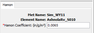
Figure 12. Entering the Hamon evapotranspiration coefficient for a subbasin.

Hargreaves

The Hargreaves evapotranspiration method (Hargreaves and Samani, 1985) is based on an empirical relationship where reference evapotranspiration was regressed with solar radiation and temperature data. The regression was based on eight years of precision lysimeter observations for a grass reference crop in Davis, CA. The method has been validated for sites around the world (Hargreaves and Allen, 2003). The method is capable of capturing diurnal variation in potential evapotranspiration for simulation time steps less than 24 hours. Combining the Hargreaves evapotranspiration method with the Hargreaves shortwave radiation method will yield the Hargreaves evapotranspiration form equivalent to Hargreavs and Allen (2003) Eq. 8.

The Hargreaves evapotranspiration method includes a Component Editor with parameter data for each individual subbasin in the meteorologic model. The Watershed Explorer provides access to the evapotranspiration component editor using a picture of a water pan (Figure 13). An air temperature gage must be selected in the atmospheric variables Component Editor for each subbasin. To open the atmospheric variables Component Editor, click on a subbasin node in the Watershed Explorer.

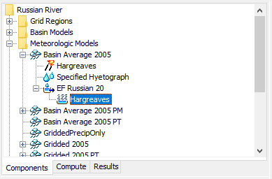
Figure 13. A meteorologic model using the Hargreaves evapotranspiration method with a component editor for each individual subbasin.

The Component Editor for each subbasin includes a Hargreaves evapotranspiration coefficient (Figure 14). A default coefficient of 0.0135 per degree Celsius is provided; this is equivalent to 0.0075 per degree Fahrenheit. If the Hargreaves evapotranspiration method is combined with the Hargreaves shortwave radiation method, the resulting default coefficient is 0.0023 per degree Celsius raised to the 3/2 power. This is equivalent to the form presented by Hargreaves and Allen (2003) Eq. 8.

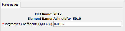
Figure 14. Entering the Hargreaves evapotranspiration coefficient for a subbasin.

Monthly Average

The monthly average method is designed to work with measured pan evaporation data. However, it can also be used with data collected with the eddy correlation technique or other modern methods. Regardless of how they are collected, the data are typically presented as the average depth of evaporated water each month. Maps or tabular reports can be found for each month and used with this method.

The monthly average method includes a Component Editor with parameter data for each individual subbasin in the meteorologic model. The Watershed Explorer provides access to the evapotranspiration component editor using a picture of a water pan (Figure 15).

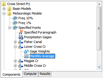
Figure 15. A meteorologic model using the monthly average evapotranspiration method with a separate component editor for each individual subbasin.

The Component Editor for each subbasin includes the evapotranspiration rate for each month of the year (Figure 16). It is entered as the total amount of evapotranspiration for the month. Every time step within the month will have the same evapotranspiration rate.
The pan coefficient must also be entered for each month. The specified rate is multiplied by the coefficient to determine the final potential rate for each month. The coefficient is usually used to correct actual evaporation pan data to more closely reflect plant water use.

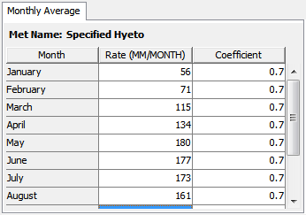
Figure 16. Entering rate and pan coefficient data for a subbasin in a meteorologic model using the monthly average evapotranspiration method.

Penman Monteith

The Penman Monteith method implements the Penman Monteith equations for computing evapotranspiration at less than a daily time interval as detailed by Allen, Pereira, Raes, and Smith (1998). The equations are based on a combination of an energy balance with a mass transfer. The maximum possible evapotranspiration is moderated by an aerodynamic resistance due to friction as air flows over the vegetation. A bulk surface resistance is added in series with the aerodynamic resistance to account for limitations to water vapor flow at the leaf surfaces and at the soil. The parameterization is entirely dependent on the atmospheric conditions.

The Penman Monteith method requires shortwave radiation and longwave radiation be included in the meteorologic model. The algorithm of Allen, Pereira, Raes, and Smith (1998) is followed most closely when the Specified Pyranograph shortwave method and the FAO56 longwave method are selected. When shortwave data is not available, Allen, Pereira, Raes, and Smith (1998) recommend using the Hargreaves shortwave method.

The Penman Monteith method includes a Component Editor with parameter data for each individual subbasin in the meteorologic model. The Watershed Explorer provides access to the evapotranspiration component editor using a picture of a water pan (Figure 17). An air temperature gage and a windspeed gage must be selected in the atmospheric variables for each subbasin. The water vapor method will require a relative humidity, dew point temperature, or air temperature gage depending on the vapor pressure type selected. To open the atmospheric variables Component Editor, click on a subbasin node in the Watershed Explorer.

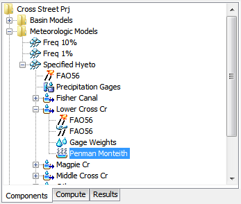
Figure 17. A model using the Penman Monteith evapotranspiration method with a component editor for each individual subbasin.

The Component Editor for each subbasin includes a selection for the vapor pressure type and reference albedo (Figure 18). Actual vapor pressure can be calculated using the dew point temperature, relative humidity, or daily minimum temperature. The daily minimum temperature option should be used when relative humidity or dewpoint data are not available; the daily minimum temperature option assumes the dewpoint temperature is equal to the daily minimum temperature. A reference albedo is required for computing the energy balance at the ground surface. A default value of 0.23 is provided.

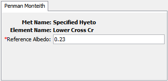
Figure 18. Entering Penman Monteith properties for a subbasin.

Priestley Taylor

The Priestley Taylor method (Priestley and Taylor, 1972) uses a simplified energy balance approach where the soil water supply is assumed to be unlimited. Simplified forms of latent and sensible energy are used. The method is capable of capturing diurnal variation in potential evapotranspiration through the use of a net solar radiation gage, so long as the simulation time step is less than 24 hours. A non-gridded shortwave radiation method should be selected in the meteorologic model. The shortwave radiation method should be configured to provide the net radiation; this is usually accomplished by computing the required value externally and inputting it using a radiation time-series gage.

The Priestley Taylor method includes a Component Editor with parameter data for each individual subbasin in the meteorologic model. The Watershed Explorer provides access to the evapotranspiration component editor using a picture of a water pan (Figure 19).
An air temperature gage must be selected in the atmospheric variables for each subbasin.

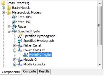
Figure 19. A meteorologic model using the Priestley Taylor evapotranspiration method with a component editor for each individual subbasin.

The Component Editor for each subbasin includes a dryness coefficient (Figure 20). The coefficient is used to make small corrections based on soil moisture state. A coefficient should be specified that represents typical soil water conditions during the simulation. A default coefficient of 1.26 is provided. This coefficient has been found to vary for regions around the world (Aschonitis, VG et al., 2017).

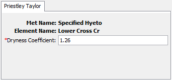
Figure 20. Entering Priestley Taylor properties for a subbasin.

Specified Evapotranspiration

The specified evapotranspiration method allows the user to specify the exact time-series to use for the potential evapotranspiration at subbasins. This method is useful when atmospheric and vegetation data will be processed externally to the program and essentially imported without alteration. This method is also useful when a single evapotranspiration observation measurement can be used to represent what happens over a subbasin.

The specified evapotranspiration method uses a Component Editor with parameter data for all subbasins in the meteorological model. The Watershed Explorer provides access to the gage component editor using a picture of a water pan (Figure 21).

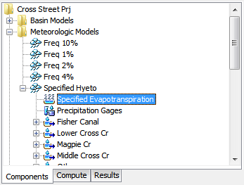
Figure 21. A meteorologic model using the specified evapotranspiration method with one component editor for subbasins.

The Component Editor for all subbasins in the meteorologic model includes the gage selection for each subbasin (Figure 22). An evapotranspiration time-series must be stored as an evapotranspiration gage before it can be used in the meteorologic model. The data may actually be from daily pan measurements, hourly eddy covariance measurements, or could be the result of complex calculations exterior to the program. Regardless, the time-series must be stored as a gage. You may use the same gage for more than one subbasin. For each subbasin in the table, select the gage to use for that subbasin. Only evapotranspiration gages already defined in the Time-Series Data Manager will be shown in the selection list.

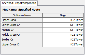
Figure 22. Selecting a time-series gage for each subbasin in a meteorologic model using the specified evapotranspiration method.