Precipitation is water falling over the land surface. It is caused when water vapor in the atmosphere condenses on airborne nuclei such as dust particles. Condensation continues to add to the droplet forming around the nuclei until the weight of the droplet exceeds the ability of wind currents to keep it aloft. Precipitation can be caused by different types of storms including stratiform, convection, and cyclone which each have typical characteristics of duration, intensity, and spatial extent. Precipitation includes the liquid form known as rain as well as a variety of frozen forms including sleet, snow, graupel, and hail. Most hydrologic purposes can be met by limiting consideration to rain and snow. The determination of the rain or snow state is made separately in the snowmelt portion of the meteorologic model.

The precipitation method included in the meteorologic model is required whenever a basin model includes subbasin elements. The options available include several that process gage measurements, a statistical method that uses depth-duration data, several design storms options, and a gridded method that can be used with radar rainfall data. Each option produces a hyetograph of precipitation falling over each subbasin. More detail about each method is provided in the following sections.

Frequency Storm

The frequency storm method is designed to produce a synthetic storm from statistical precipitation data. The most common source of statistical data in the United States is the National Weather Service. Typically, the data is given in the form of maps, where each map shows the expected precipitation depth for a storm of specific duration and exceedance probability. This method is designed to use data collected from the maps along with other information to compute a hyetograph for each subbasin.

The frequency storm method includes a Component Editor with parameter data for all subbasins in the meteorologic model, and a separate Component Editor for each individual subbasin. The Watershed Explorer provides access to the precipitation component editors using a picture of raindrops (Figure 1).

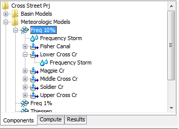
Figure 1. A meteorologic model using the frequency precipitation method with a Component Editor for all subbasins, and a separate Component Editor for each individual subbasin.

The Component Editor for all subbasins in the meteorologic model includes parameter data to describe the frequency storm (Figure 3). The frequency storm method is designed to accept partial or annual-duration precipitation depth-duration data. A conversion factor, or "Annual-Partial Ratio", can be applied when the output, computed flow, is required to be different than the input precipitation. The difference between frequency curves derived from partial and annual-duration information is extremely small for exceedance probabilities 4% and smaller; annual and partial duration frequency curves usually converge beyond the 10% exceedance probability. Adjustment factors are available for annual-partial duration differences for the 10%, 20% or 50% exceedance probabilities. Figure 2 shows the available options for annual to partial duration adjustments. Once the Annual-Partial Conversion option is selected in the list, the Annual-Partial Ratio field is automatically populated with a ratio that is appropriate to the user specified "Annual-Partial Conversion" option. By default, the None Annual-Partial Conversion option is selected and a ratio of 1.0 is applied to the precipitation frequency information. If the 50 Percent Annual to Partial option is selected, then a ratio of 1.14 is applied to the precipitation frequency information, converting it from an annual duration frequency curve to a partial duration frequency curve. If the 50 Percent Partial to Annual option is selected, then a ratio of 0.88 is applied to the precipitation frequency information, converting it from partial duration frequency curve to an annual duration frequency curve.

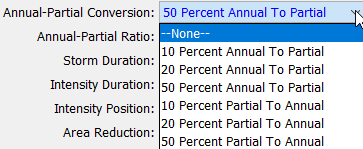
Figure 2. Options available for converting between annual and partial duration frequency information.

The storm duration determines how long the precipitation will last. The storm duration must be longer than the intensity duration. Historic storms within the region can aid in setting an appropriate storm duration. The intensity duration specifies the shortest time period of the storm. Usually the intensity duration should be set equal to the time step of the simulation. It must be less than the total storm duration. If the simulation duration is longer than the storm duration, then all time periods after the storm duration will have zero precipitation.

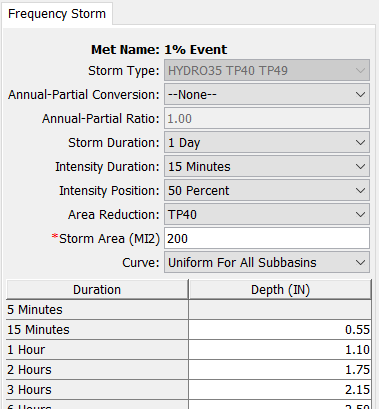
Figure 3. Precipitation editor for all subbasins when the frequency storm method is selected.

The intensity position determines where in the storm the period of peak intensity will occur. Changing the position does not change the total preciptation depth of the storm, but does change how the total depth is distributed in time during the storm. You may select 25%, 33%, 50%, 67%, or 75% from the list of choices. If the storm duration is selected to be 6 hours and the 25% position is selected, the peak intensity will occur 1.5 hours after the beginning of the storm. The default selection is 50%.

The area reduction determines the area-reduction curves for reducing point precipitation, precipitation at a gage, to precipitation over a storm area. There are two options, None and TP40. Future versions of HEC-HMS will include a user option where user defined area-reduction curves can be applied to each storm duration precipitation value. The None area reduction method would be selected if the user already applied area reduction factors to the precipitation frequency information, or if the user did not want area-reduction factors to be applied to the analysis. The TP40 area reduction option will result in the program applying the area-reduction curves in NOAA Technical Paper Number 40 (TP 40). There are different area-reduction curves for different storm durations.

The storm area is only required if the TP40 area reduction option is selected. When the TP40 option is selected, then the storm area is used to automatically compute the depth-area reduction factor for each storm duration. In most cases the specified storm area should be equal to the watershed drainage area at the point of evaluation. The same hyetograph is used for all subbasins. A storm area value must be entered by the user, the storm area can not be left empty. The depth-area analysis simulation can be used to quickly analyze multiple analysis points (the user chooses the analysis points). The depth-area analysis simulation is a multi-compute simulation where the storm area, precipitation hyetograph, and runoff is compute for each analysis point.

Precipitation depth values must be entered for all durations from the peak intensity to the total storm duration. Values for durations less than the peak intensity duration, or greater than the total storm duration are not entered. Values should be entered as the cumulative precipitation depth expected for the specified duration.

The Component Editor for each individual subbasin in the meteorologic model is used to specify a separate depth-duration curve for each subbasin (Figure 4). The depth-duration curve can only be entered for a subbasin if the "Curve" option (Figure 3) is set to Variable by Subbasin. Using this option may be necessary if the watershed is large and the depth-duration characteristics of the precipitation change significantly over the watershed. For example, mountainous areas may have changes in the precipitation characteristics with changes in elevation.

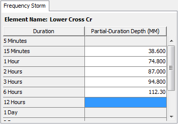
Figure 4. Entering a separate depth-duration curve for each subbasin.

Gage Weights

The gage weights method is designed to work with recording and non-recording precipitation gages. Recording gages typically measure precipitation as it occurs and then the raw data are converted to a regular time step, such as 1 hour. Non-recording gages usually only provide an estimate of the total storm depth. The user can choose any method to develop the weights applied to each gage when calculating the hyetograph for each subbasin. For increased flexibility, the total storm depth and the temporal pattern are developed separately for each subbasin. Optionally, an index depth can be assigned to each gage and subbasin. The index is used to adjust for regional bias in annual or monthly precipitation.

The gage weights method includes several options for processing precipitation gage data (Figure 5). The indexing option is used to adjust gage data when there are regional trends in precipitation patterns. Using the index option requires the specification of an index value for each precipitation gage and each subbasin. The average annual precipitation total is often used as the index at a gage, and the estimated average annual precipitation over a subbasin area is often used as the index for a subbasin. Alternately, the monthly average values may be used at each gage and each subbasin. The index values are used to adjust the precipitation data for regional trends before calculating the weighted depth and weighted timing. The total override option is used to adjust the precipitation depth at each gage. Without the override, the total depth at a gage is the sum of the values in the gage record. With the override, the values in the gage record are proportionally adjusted to have a sum equal to the specified total value.

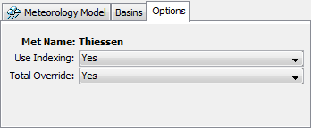
Figure 5. Selecting options for the gage weights precipitation method.

The gage weights method includes a Component Editor with parameter data for all subbasins in the meteorologic model. A Component Editor is also included for specifying the parameter data for precipitation gages. Finally, a separate Component Editor is included for each individual subbasin in the meteorologic model. The Watershed Explorer provides access to the precipitation component editors using a picture of raindrops, and provides access the gage component editor using a picture of a measurement gage (Figure 6).

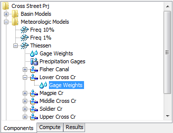
Figure 6. A meteorologic model using the gage weights precipitation method with a component editor for all subbasins, a component editor for precipitation gages, and a separate Component Editor for each individual subbasin.

The Component Editor for all subbasins in the meteorologic model includes the optional index for each subbasin. The parameter data for indexing is only entered when the option is activated (Figure 5). In order to use the optional index, an index value must be entered for each subbasin and precipitation gage.

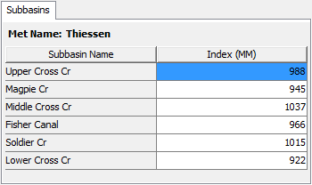
Figure 7. Specifying indices for each subbasin using average annual precipitation depth. Other methods may be used to estimate the index.

The Component Editor for all precipitation gages in the meteorologic model includes the optional total depth override and optional indexing. The parameter data for override and indexing is only entered when the respective options are activated (Figure 5). The optional total depth override is entered for each gage (Figure 8). If no total depth is entered, the depth will be the sum of the data actually stored in the precipitation gage. However, if a total depth is entered, the exact pattern is maintained but the magnitude of precipitation at each time step is adjusted so that the specified depth is applied over the entire simulation. Total depth can be specified for no precipitation gages, one gage, many gages, or all gages. Turning off the "Use Override" option will remove all total depth data for time-series precipitation gages.

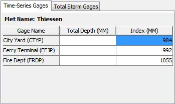
Figure 8. Entering optional total depth and index for the precipitation gages.

The optional index is entered for each gage. If you enter an index for a gage, it can only be used during a simulation if you also specify an index for all gages used in a subbasin and also specify an index for the subbasin. Turning off the "Use Indexing" option will remove all indexes from the meteorologic model.

Total storm gages are created and managed directly from the meteorologic manager. To create a new total storm gage, access the "Total Storm Gages" tab and enter a gage name in the first column of the last row (Figure 9). The last row is always kept blank for creating new gages. You can rename a gage by typing over the name in the first column. You can delete a gage by deleting its name from the first column and any data from the other columns. You must always enter a total depth for the gage that represents the total precipitation during the simulation.

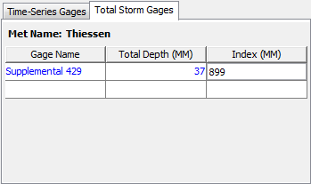
Figure 9. Creating a total storm gage and entering the total storm depth and optional index.

The Component Editor for each subbasin in the meteorologic model is used to select the precipitation gages for that subbasin and to enter weights for each selected gage (Figure 10). The "Gage Selections" tab is where the gages are selected. All of the available gages are shown in a table. The available gages are the precipitation time-series gages defined in the Time-Series Data Manager plus any total storm gages defined in the meteorologic model. For each subbasin you must separately select which gages will be used for that subbasin.

The "Gage Weights" tab is where the weights are specified for each gage selected for a subbasin (Figure 11). The gages are shown in a table with a separate row for each gage. Only the gages selected previously on the "Gage Selections" tab are included in the table. For each gage you can enter a depth weight. You can enter a time weight for time-series gages. The values entered for the depth or time weights are automatically normalized during the simulation. The value of the weights must be estimated separate from the program. Possible methods for computing the weights include Thiessen polygons, inverse distance, inverse distance squared, isohyetal mapping, or any method deemed appropriate.

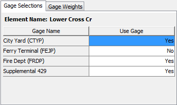
Figure 10. Selecting which gages to use for a subbasin.

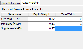
Figure 11. Entering depth and time weights for the selected gages.

Gridded Precipitation

The gridded precipitation method is designed to work with the ModClark gridded transform. However, it can be used with other area-average transform methods as well. The most common use of the method is to utilize radar-based precipitation estimates. Using additional software, it is possible to develop a gridded representation of gage data or to use output from atmospheric models. If it is used with a transform method other than ModClark, an area-weighted average of the grid cells in the subbasin is used to compute the precipitation hyetograph for each subbasin.

The gridded precipitation method includes a Component Editor with parameter data for all subbasins in the meteorologic model. The Watershed Explorer provides access to the precipitation component editor using a picture of raindrops (Figure 12).

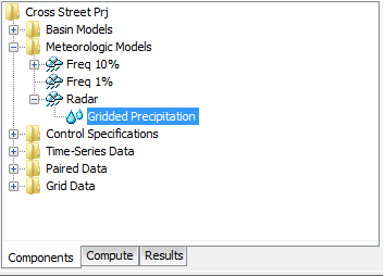
Figure 12. A meteorologic model using the gridded precipitation method with a Component Editor for all subbasins.

The Component Editor for all subbasins in the meteorologic model includes parameter data to describe the gridded precipitation (Figure 13). Gridded precipitation data must be stored as a precipitation grid before it can be used in the meteorologic model. The data may be from radar sources or could be the result of complex calculations exterior to the program. Regardless, the grid data must be stored as a precipitation grid. Only precipitation grids already defined will be shown in the selection list.

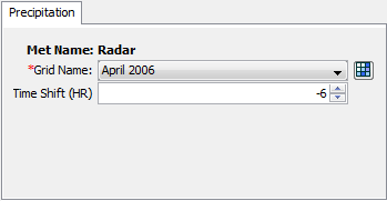
Figure 13. Precipitation component editor for the gridded precipitation method.

The time shift can be used to correct for precipitation grids stored with a time zone offset. All calculations during a simulation are computed assuming an arbitrary local time zone that does not observe summer time (daylight savings in the United States). It is common for precipitation data from radar sources to be referenced in Coordinated Universal Time (UTC). Set the shift to zero if all the time-series and grid data is referenced in same local time zone. If other data sources such as observed discharge or temperature are referenced in local time and the precipitation grid is in UTC, select the correct shift so that the precipitation data will match the rest of the data. Local time zones located to the West of the zero longitude line will use a positive shift when the precipitation grid is referenced in UTC. Local time zones located to the East of the zero longitude line will use a negative shift when the precipitation grid is referenced in UTC.

HMR 52 Storm

The HMR 52 storm is one approach to computing the probable maximum precipitation for a watershed as detailed in Hydrometeorological Report No 52 (Hansen, Schreiner, and Miller, 1982). Concentric ellipses are used to construct the storm spatial pattern where each ellipse represents an isohyet of precipitation depth. The storm is located over the watershed by specifying the center of the pattern and the angle of the major axis of the ellipses. Total precipitation depth is computed using a specified storm area and area-duration precipitation curves. The total precipitation depth is converted to a temporal pattern based on the selected placement of the peak intensity within the storm duration. The most intense 6-hour period of the storm is constructed using the ratio of precipitation depth between the largest and sixth-largest hours.

HEC-HMS computes the precipitation hyetograph for each subbasin intersecting the polygon outline of the subbasin with the storm. The geometric data for the polygon outline comes from the same source as GIS features (See Drawing Elements and Labels). It is optional to use GIS features for drawing subbasin elements in the Basin Map. However, the subbasin GIS features become required for using the HMR 52 storm.

The HMR 52 storm method includes several parameters to describe the location, orientation, and temporal distribution of the storm plus additional information on the area reduction (Figure 14). The X and Y coordinate parameters are used to specify the center of the storm pattern. The coordinate values should be entered using the same coordinate system as the geometric data for the subbasin polygons. The preferred orientation is measured in degrees increasing clockwise from north. The actual orientation is also measured in degrees increasing clockwise from North. Following guidelines in Hydrometeorological Report No 52 (HMR 52), a reduction is applied when the actual orientation deviates from the preferred orientation by more than 40 degrees. As stated in HMR52, the storm orientation should be bounded by 135 and 315 degrees.

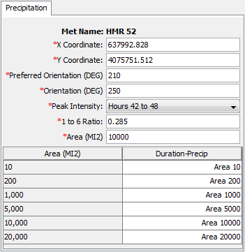
Figure 14. Precipitation component editor for the HMR 52 storm.

The HMR 52 storm is 72 hours long and begins at the simulation start time. The peak intensity parameter specifies the period within the 72-hour storm when the precipitation rate will be greatest. The 6-hour period of peak intensity can be set to begin as early as hour 24 of the storm or as late as hour 60 of the storm. The depth of rain falling during the period of peak intensity is subdivided into 1-hour increments using the parameter for the ratio of the 1-hour to 6-hour depth.

The total storm area must be specified. Additionally, a duration-precipitation function must be selected for the range of possible storm areas. In general, the curves are constructed using data available in Hydrometeorological Report No 51 (Schreiner and Riedel, 1978). Each duration-precipitation function must be defined in the paired data manager before it can be selected. You can press the paired data button next to the selection list to use a chooser. The chooser shows all of the available duration-precipitation functions in the project.

The HMR 52 storm method creates a storm from input specified by the user including storm center, orientation, and area. The optimization trial compute option can be used to automatically select these parameters in order to maximize peak runoff, or volume, or reservoir pool elevation.

Inverse Distance

The inverse distance method was originally designed for application in real-time forecasting systems. It can use recording gages that report on a regular interval like 15 minutes or 1 hour. It can also use gages that only report daily precipitation totals. Because it was designed for real-time forecasting, it has the ability to automatically switch from using close gages to using more distant gages when the closer gages stop reporting data. The latitude and longitude of the gages is used to determine closeness to one or more nodes specified in each subbasin. The distance at which gages are used for a subbasin is controlled by the search distance. Optionally, an index depth can be assigned to each gage and subbasin node. The index is used to adjust for regional bias in annual or monthly precipitation.

The inverse distance method includes several options for processing precipitation gage data (Figure 15). The indexing option is used to adjust gage data when there are regional trends in precipitation patterns. Using the index option requires the specification of an index value for each precipitation gage and each node in each subbasin. The average annual precipitation total is often used as the index at a gage, and the estimated average annual precipitation at a node location is often used as the index for a subbasin node. Alternately, the monthly average values may be used at each gage and each node. The search distance option can be used to limit the influence distance of precipitation gages. When no search distance is specified, the default value of 1,000 kilometers is used. When an optional distance is entered, gages are only used at a subbasin node if they are within the specified distance.

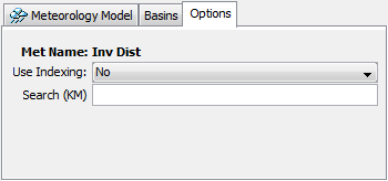
Figure 15. Selecting options for the inverse distance precipitation method.

The inverse distance method includes a Component Editor for specifying the parameter data for precipitation gages. A Component Editor is also included for each individual subbasin in the meteorologic model. The Watershed Explorer provides access to the gage component editor using a picture of a measurement gage, and provides access the the precipitation component editor for each subbasin with a picture of raindrops (Figure 16).

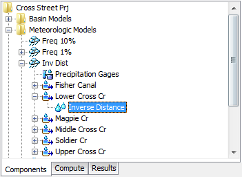
Figure 16. A meteorologic model using the inverse distance precipitation method with a component editor for precipitation gages and a separate component editor for each individual subbasin.

The Component Editor for all precipitation gages in the meteorology model is used to select gages for processing, control how they are processed, and enter optional indexing parameter data (Figure 17). All gages used in the inverse distance method must be setup in the Time-Series Data Manager before they can be used. The Component Editor will subsequently show all available precipitation gages. You may determine which gages will be used in the meteorology model by setting the appropriate choice in the "Use Gage" column.

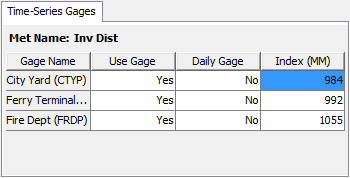
Figure 17. Selecting which time-series gages to use for a subbasin included in a meteorologic model with the inverse distance precipitation method selected. The index precipitation is optional.

Each precipitation gage may use any of the allowable time intervals from 1 minute to 24 hours. When a gage is selected as a daily gage, it is assumed during calculations that the daily precipitation depth is known but there is no timing information. Usually daily gages are stored with a 24-hour time interval, but any interval may be used. Daily gage data is only used during processing for days where the entire day is within the simulation time window. When a gage is not selected as a daily gage, the data it contains is interpolated to the simulation time step. The appropriate setting should be made in the "Daily Gage" column.

The optional index is entered for each gage. If you enter an index for a gage, it can only be used during a simulation if you also specify an index for all gages used in a subbasin and also specify an index for each node in that subbasin. Turning off the "Use Indexing" option will remove all indexes from the meteorologic model.

The Component Editor for each subbasin in the meteorologic model is used to create one or more nodes and enter the coordinates for each node (Figure 18). A minimum of one node is required. To create a new node, access the "Node Weights" tab and enter a node name in the first column of the last row. The last row is always kept blank for creating new nodes. You can rename a node by typing over the name in the first column. You can delete a node by deleting its name from the first column and any data from the other columns. You must always enter a weight for a node. The weight controls how the final hyetograph is computed for the subbasin from the hyetographs computed at each node. If you have enabled the indexing option, you should also enter the index for each node. The index is used to adjust for regional bias in annual or monthly precipitation.

All nodes that you have created will be shown on the "Latitudes" and "Longitudes" tabs. You must enter the appropriate coordinate information for each node. Coordinates may be entered using degree-minute-second format or alternately may be entered using decimal degree format. The data entry format is selected in the Program Settings.

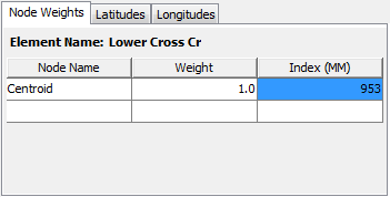
Figure 18. Creating an inverse distance node in a subbasin.

Hypothetical Storm

The Hypothetical Storm replaced the SCS Storm method available in HEC-HMS version 4.2.1 and prior versions. The hypothetical storm is a general approach that allows users to enter the storm duration, depth, area reduction information, the temporal pattern, and storm area. The Hypothetical Storm method includes a Component Editor with parameter data for all subbasins in the meteorologic model. The Watershed Explorer provides access to the precipitation component editor using a picture of raindrops (Figure 19).

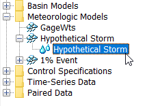
Figure 19. A meteorologic model using the Hypothetical Storm precipitation method with one component editor for all subbasins.

The Component Editor for all subbasins in the meteorologic model specifies the parameter data for the storm (Figure 20). The "Method" selection is required to set the temporal pattern approach for the hypothetical storm.  Options include the 4 standard SCS temporal patterns (SCS Type 1, SCS Type 1A, SCS Type 2, and SCS Type 3), a user-specified pattern, and an area-dependent temporal pattern.  Figure 20 shows the User-Specified Pattern option selected for the method.  When this option is selected, the user must define the "Storm Pattern" and the "Storm Duration" in addition to the depth and area-reduction information. The user defined "Storm Pattern" is entered as a percentage curve in the Paired Data Manager. The independent variable is percent of the total storm duration (values should be 0 to 100 percent) and the dependent value is percent of the point depth (which is automatically reduced based on the area-reduction information and storm area). The 4 standard SCS temporal patterns are built into HEC-HMS. Each of the SCS storms are 24 hours long. The simulation must have a duration of 24 hours or longer. All precipitation values after the first 24 hours will be zero. The Area-Dependent Pattern option is designed to work in conjunction with the Depth-Area analysis compute option. When Area-Dependent Pattern is selected, the user must define a number of storm temporal patterns for different storm areas. HEC-HMS interpolates between the temporal patterns using the user defined storm area, or the area for an analysis point in the Depth-Area analysis.  

The user can define the storm depth and area-reduction information after the temporal pattern is selected. There are two options for specifying the storm depth under the "Precipitation Method." The first is "Point Depth", which requires the user to enter a single point depth value that will be used for every subbasin in the meteorologic model. The user must also specify a storm area when using the "Point Depth" method. The second option is "Precipitation-Frequency Grid" (Figure 21), where the user can specify a Precipitation-Frequency Grid, created as a grid dataset. The user must also specify a computation point for this method. This method can only be used with georeferenced basin models, because HEC-HMS will automatically intersect the precipitation-frequency grid with the sub-basin polygons to compute the basin-average precipitation value, as well as automatically compute the storm area, equal to the drainage area above the computation point.

There is an "Area Reduction" method, the user can choose between None, TP40, and User-Specified. The None options means the "Point Depth" or "Precipitation-Frequency Grid" will be used to compute the subbasin hyetograph. The 24-hour area reduction curve from TP40 is used when TP40 is selected for the area-reduction method. The TP40 area reduction method should only be selected when one of the SCS temporal patterns is selected or when a 24-hour Storm Duration with a User-Specified temporal pattern is selected. A "Storm Area" is required for both the TP40 and User-Specified area reduction options. HEC-HMS will interpolate the reduction factor from the TP40 or User-Specified area reduction curve to update the storm depth.  

The Hypothetical Storm will work with the Depth-Area Analysis compute option, similar to the frequency storm precipitation method. The drainage area at each of the user-defined analysis points will replace the storm area during the depth-area analysis simulation. The appropriate temporal pattern and precipitation depth are computed for each storm area when the area-dependent temporal pattern option is selected. When the "Precipitation-Frequency Grid" precipitation method is used, the Depth-Area Analysis will compute the basin-average precipitation from the grid for each computation point as well. The Depth-Area Analysis will also override any computation point selected in the Hypothetical Storm precipitation method and only use those specified in the Depth-Area Analysis.

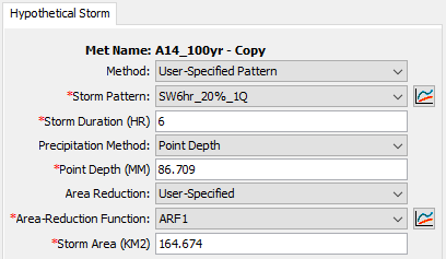
Figure 20. Precipitation component editor for the Hypothetical Storm precipitation method, with Point Depth precipitation specification.

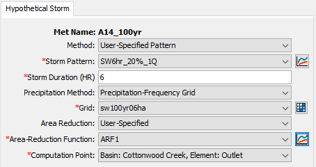
Figure 21. Precipitation component editor for the Hypothetical Storm precipitation method, with Precipitation-Frequency Grid precipitation specification.

Specified Hyetograph

The specified hyetograph method allows the user to specify the exact time-series to use for the hyetograph at subbasins. This method is useful when precipitation data will be processed externally to the program and essentially imported without alteration. This method is also useful when a single precipitation gage can be used to represent what happens over a subbasin.

The specified hyetograph method includes an option for processing precipitation gage data (Figure 22). The total override option is used to adjust the precipitation depth at each gage. Without the override, the total depth at a gage is the sum of the values in the gage record. With the override, the values in the gage record are proportionally adjusted to have a sum equal to the specified total value.

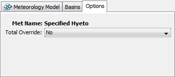
Figure 22. Selecting options for the specified hyetograph precipitation method.

The specified hyetograph method uses a Component Editor with parameter data for all subbasins in the meteorological model. The Watershed Explorer provides access to the component editor using a picture of raindrops (Figure 23).

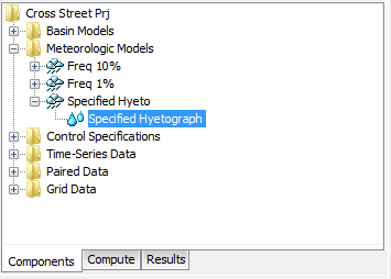
Figure 23. A meteorologic model using the specified hyetograph precipitatiom method with a component editor for all subbasins.

The Component Editor for all subbasins in the meteorologic model includes the gage selection for each subbasin and the optional depth override for each subbasin (Figure 24). A hyetograph must be stored as a precipitation gage before it can be used in the meteorologic model. The data may actually be from a recording gage or could be the result of complex calculations exterior to the program. Regardless, the hyetograph must be stored as a gage. You may use the same gage for more than one subbasin. For each subbasin in the table, select the gage to use for that subbasin. Only precipitation gages already defined in the Time-Series Data Manager will be shown in the selection list.

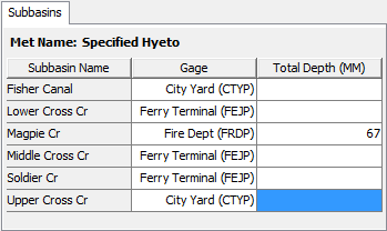
Figure 24. Selecting a gage for each subbasin. Total depth override is optional.

Optionally, you may enter a total depth for each subbasin. If no total depth is entered, the depth will be the sum of the data actually stored in the precipitation gage. However, if a total depth is entered for a subbasin, the exact pattern is maintained but the magnitude of precipitation at each time step is adjusted proportionally so that the specified depth is applied over the entire simulation. Total depth can be specified for no subbasins, one subbasin, many subbasins, or all subbasins. It is not required to enter the depth for all subbasins in order to specify it for just one subbasin.

Standard Project Storm

The standard project storm method implements the requirements of Engineering Manual EM-1110-2-1411 (Corps 1965). While the methodology is no longer frequently used, it is included in the program for projects where it may still necessary.

The standard project storm method includes a Component Editor with parameter data for all subbasins in the meteorologic model. The Watershed Explorer provides access to the precipitation component editors using a picture of raindrops (Figure 25).

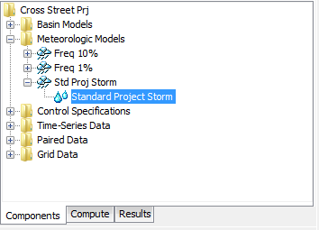
Figure 25. A meteorologic model using the standard project storm method with a component editor for all subbasins.

The Component Editor for all subbasins in the meteorologic model includes parameter data to describe the storm (Figure 26). The precipitation index represents the depth of rainfall during the storm. This index is not the same as the probable maximum precipitation and does not have an associated exceedance probability. The index in selected from a map in the Engineering Manual.

The storm area is used to automatically compute the depth-area reduction factor, based on figures in the Engineering Manual. In most cases the specified storm area should be equal to the watershed drainage area at the point of evaluation.

The distribution determines how the adjusted precipitation depth for each subbasin is shaped into a hyetograph; it must be selected from the list of available choices. The Standard option uses the procedure specified in the Engineering Manual to distribute the adjusted storm depth. The Southwest Division option uses a different procedure that may be more applicable in some watersheds.

The transposition factor accounts for the location of a subbasin in the watershed, relative to the center of the storm (Figure 27). The Engineering Manual contains an isohyetal map with concentric rings labeled in percent. If a subbasin is generally covered by the 120% isohyetal line, then a factor of 1.20 should be entered in the program.

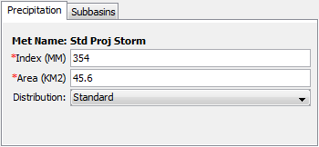
Figure 26. Entering properties of the standard project storm.

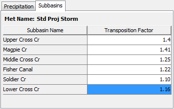
Figure 27. Entering a transposition factor for each subbasin.