The program is designed with reusable data sets that can be independently developed. However, some data sets depend on others for important definitions. For example, gages must be created before they can be used in basin or meteorologic models. Consequently, there is a necessary sequence to successfully obtain results. The remainder of this chapter provides an overview of the best procedure for obtaining computation results.

Create a New Project

Create a new project by selecting the File | New… menu command. After you press the button a window will open where you can name, choose a location on your computer or a network computer to save the new project, and enter a description for the new project. If the description is long, you can press the button to the right of the description field to open an editor. You should also select the default unit system; you can always change the unit system for any component after it is created but the default provides convenience. Press the Create button when you are satisfied with the name, location, and description. You cannot press the Create button if no name or location is specified for the new project. If you change your mind and do not want to create a new meteorologic model, press the Cancel button or the X button in the upper right of the Create a New Project window.

Enter Shared Project Data

Shared data includes time-series data, paired data, and grid data. Shared data is often required by basin and meteorologic models. For example, the meteorologic model typically requires precipitation observations. In another example, a reach element using the Modified-Puls routing method requires a storage-discharge relationship for the program to calculate flow through the reach. The following is a complete list of shared data types used by the program.

All of the different types of time-series data:

• Precipitation
• Discharge
• Stage
• Temperature
• Radiation
• Windspeed
• Air pressure
• Humidity
• Altitude
• Crop coefficient
• Snow water equivalent
• Sediment load
• Concentration
• Percent
• Evapotranspiration
• Sunshine

All of the different types of paired data:

• Storage-discharge
• Elevation-storage
• Elevation-area
• Elevation-discharge
• Inflow-diversion
• Diameter-percentage
• Cross sections
• Inflow-lag
• Outflow-attenuation
• Elevation-width
• Elevation-perimeter
• Area-reduction
• Unit hydrograph curves
• Percentage curves
• Duration-precipitation
• ATI-meltrate
• ATI-coldrate
• Groundmelt patterns
• Percent patterns
• Cumulative probability
• Parameter value sample

All of the different types of grid data:

• Precipitation
• Temperature
• Radiation
• Crop coefficient
• Storage capacity
• Percolation rate
• Storage coefficient
• Moisture deficit
• Impervious Area
• SCS curve number
• Elevation
• Cold content
• Cold content ATI
• Meltrate ATI
• Liquid water content
• Snow water equivalent
• Water content
• Water potential
• Air pressure
• Humidity
• Windspeed

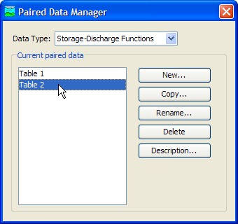
Open a component manager to add shared data to a project. Go to the Components menu and select Time-Series Data Manager, Paired Data Manager, or Grid Data Manager command. Each one of these component managers contains a menu for selecting the type of data to create or manage. The Paired Data Manager with the Storage-Discharge data type selected is shown in Figure 1. Once the data type is selected, you can use the buttons on the right side of the component manager to add a New, Copy, Rename, and Delete a data type. There is also a button that opens an editor where you can change the description of the selected component. In the case of time-series data, the manager contains two extra buttons to add or delete time windows. A time window is needed for entering or viewing time-series data.

Describe the Physical Watershed

The physical watershed is represented in the basin model. Hydrologic elements are added and connected to one another to model the real-world flow of water in a natural watershed. A description of each hydrologic element is given in the Table below.

The basin model manager can be used to add a new basin model to the project. Open the basin model manager by selecting the Components | Basin Model Manager command. The basin model manager can be used to copy, rename, or delete an existing basin model.

Hydrologic elements can be added to the basin map after it is created. Select the basin model in the Watershed Explorer to open the basin map. If background map layers are available, add them to the basin model before adding elements. Add an element by selecting one of the tools from the toolbar, and clicking the left mouse button on the desired location in the basin map. Connect an element to a downstream element by right-clicking the upstream element to access the Connect Downstream menu item.

Most hydrologic elements require parameter data so that the program can model the hydrologic processes represented by the element. In the case of the subbasin element, many mathematical models are available for determining precipitation losses, transforming excess precipitation to streamflow at the subbasin outlet, and adding baseflow. In this document the different mathematical models will be referred to as methods. The available methods for subbasin and reach elements are shown in the Table below.

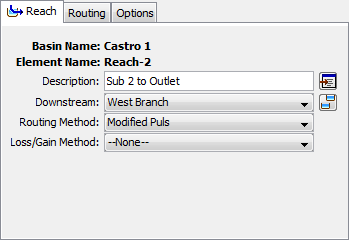
Parameter data is entered in the Component Editor. Select a hydrologic element in the basin map or Watershed Explorer to open the correct Component Editor as shown in the Figure below.

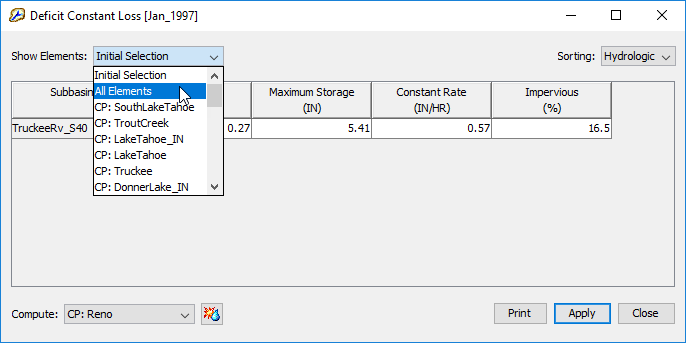
Global parameter editors can also be used to enter or view parameter data for many hydrologic elements as shown in the Figure below. Global parameter editors are opened using the Parameters menu.

Describe the Meteorology

The meteorologic model calculates the precipitation input required by a subbasin element. The meteorologic model can utilize both point and gridded precipitation and has the capability to model frozen and liquid precipitation along with evapo-transpiration. The snowmelt methods model the accumulation and melt of the snow pack. The evapo-transpiration methods include the constant monthly, Priestley Taylor, and Penman Monteith methods, with gridded options available. An evapo-transpiration method is only required when simulating the continuous or long term hydrologic response in a watershed. When an energy balance evapo-transpiration or snowmelt method is selected, the shortwave and longwave radiation must also be specified. A brief description of the methods available for calculating basin average precipitation or grid cell precipitation is included in the Table.

Use the meteorologic model manager to add a new meteorologic model to the project. Go to the Components menu and select the correct option from the menu list. The meteorologic model manager can also be used to copy, rename, and delete an existing meteorologic model.

Enter Simulation Time Windows

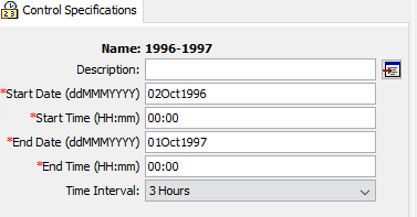
A simulation time window sets the time span and time interval of a simulation run. A simulation time window is created by adding a control specifications to the project. This can be done using the control specifications manager. Go to the Components menu and select the correct option from the menu list. Besides creating a new simulation time window, the control specifications manager can be used to copy, rename, and delete an existing window.

Once a new control specifications has been added to the project, use the mouse pointer and select it in the Watershed Explorer. This will open the Component Editor for the control specifications as shown in Figure 4. Information that must be defined includes a starting date and time, ending date and time, and time interval. The grid data output interval and grid time shift are specific to simulations that included gridset data.

Simulate and View Results

A simulation run calculates the precipitation-runoff response in the basin model given input from the meteorologic model. The control specifications define the time period and time interval. All three components are required for a simulation run to compute.

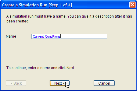
Create a new simulation run by selecting the Compute | Create Simulation Run menu option. A wizard will open to step you through the process of creating a simulation run as shown in the Figure. First, enter a name for the simulation. Then, choose a basin model, meteorologic model, and control specifications. After the simulation run has been created, select the run. Go to the Compute | Select Run menu option. When the mouse moves on top of Select Run a list of available runs will open. Choose the correct simulation. To compute the simulation, re-select the Compute menu and choose the Compute Run option at the bottom of the menu.

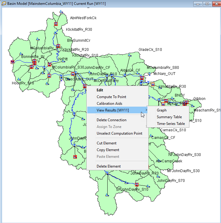
Results can be accessed from the basin map and the Watershed Explorer, "Results" tab. Results are available as long as a simulation run has been successfully computed and no edits have been made after the compute to any component used by the simulation run. For example, if the time of concentration parameter was changed for a subbasin element after the simulation run was computed, then results are no longer valid for that hydrologic element and any elements downstream of it in the basin model. The simulation run must be recomputed for results to update.

The simulation must be selected (from the Compute menu or Watershed Explorer) before results can be accessed from the basin map. After the simulation run is selected, select the hydrologic element where you want to view results. While the mouse is located on top of the element icon, click the right mouse button. In the menu that opens, select the View Results option. Three result types are available: Graph, Summary Table, and Time-Series Table.

These results can also be accessed through the toolbar and the Results menu. A hydrologic element must be selected before the toolbar buttons and options from the Results menu are active. A global summary table is available from the toolbar and Results menu. The global summary table contains peak flows and time of peak flows for each hydrologic element in the basin model.

Results can also be viewed from the Watershed Explorer, "Results" tab. Select the simulation run and the Watershed Explorer will expand to show all hydrologic elements in the basin model. If you select one of the hydrologic elements, the Watershed Explorer expands again to show all result types as shown in the Figure.

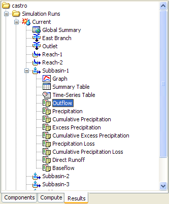
For a subbasin element, you might see outflow, incremental precipitation, excess precipitation, precipitation losses, direct runoff, and baseflow as the output results. Select one of these results to open a preview graph. Multiple results can be selected and viewed by holding down the Control or Shift buttons. Results from multiple hydrologic elements can be viewed together. Also, results from different simulation runs can be selected and viewed. Once output types are selected in the Watershed Explorer, a larger graph or time-series table can be opened in the Desktop by selecting the Graph and Time-Series buttons on the toolbar.

Create or Modify Data

Many hydrologic studies are carried out to estimate the change in runoff given some change in the watershed. For example, a residential area is planned in a watershed. The change in flow at some point downstream of the new residential area is required to determine if flooding will occur as a result of the new residential area. If this is the case, then two basin models can be developed. One is developed to model the current rainfall-runoff response given predevelopment conditions and another is developed to reflect future development.

An existing basin model can be copied using the basin model manager or the right mouse menu in the Watershed Explorer. In the Watershed Explorer, "Components" tab, select the basin model. Keep the mouse over the selected basin model and click the right mouse button. Select the Create Copy… menu item to copy the selected basin model. The copied basin model can be used to model the future development in the watershed.

To reflect future changes in the watershed, method parameters can be changed. For example, the percent impervious area can be increased for a subbasin element to reflect the increase in impervious area from development. Routing parameters can also be adjusted to reflect changes to the routing reach.

Make Additional Simulations and Compare Results

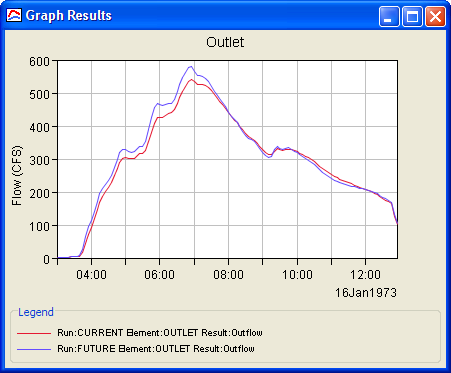
Additional simulations can be created using new or modified model components. Results from each simulation run can be compared to one another in the same graph or time-series table. Select the "Results" tab in the Watershed Explorer. Select each simulation run that contains results you want to compare. The Watershed Explorer will expand to show all hydrologic elements in the basin models. Select the hydrologic element in all simulation runs where results are needed. This will expand the Watershed Explorer even more to show available result types. Press the Control key and select each output result from the different simulation runs. When a result type is selected the result is added to the preview graph. Once all the results have been selected, a larger graph or time-series table can be opened by selecting the Graph and Time-Series buttons on the toolbar as seen in the Figure.

Exit the Program

Save the project by selecting the File | Save menu item. After the project is saved, exit the program by selecting the File | Exit menu item.