Download PDF
Download page Time-Series Data.
Time-Series Data
Hydrologic models often require time-series of precipitation data for estimating basin-average rainfall. A time-series of flow data, often called observed flow or observed discharge, is helpful for calibrating a model and is required for optimization. Other kinds of time-series data are used as well. Time-series data is stored in a project as a gage. The program separates different types of data with different gage types. Gage data only has to be entered one time. The gages are part of the project and can be shared by multiple basin or meteorologic models.
Creating a New Gage
A new gage is created using the Time-Series Data Manager. To access the manager, click on the Components menu and select the Time-Series Data Manager menu command (Figure 1). The manager can remain open while you perform tasks elsewhere in the program. You can close the manager using the X button in the upper right corner. At the top of the manager is a Data Type menu. This option lets you select one of the time-series data types supported by the program. Refer to Table 2 for a complete list of time-series data types. When a data type is selected, the manager will show all time-series data of the same type. The buttons to the right of the time-series data list can be used to manage existing data or create new data.

To create a new time-series gage, press the New… button. After you press the button a window will open (Figure 2) where you can name and describe the new gage. A default name is provided for the new gage; you can use the default or replace it with your own choice. A description can also be entered. If the description is long, you can press the button to the right of the description field to open an editor. The editor makes it easy to enter and edit long descriptions. When you are satisfied with the name and description, press the Create button to finish the process of creating the new time-series gage. You cannot press the Create button if no name is specified. If you change your mind and do not want to create a new time-series gage, press the Cancel button or the X button in the upper right to return to the time-series data manager.

Copying a Gage
There are two ways to copy a time-series gage. Both methods for copying a gage create an exact duplicate with a different name. Once the copy has been made it is independent of the original and they do not interact.
The first way to create a copy is to use the Time-Series Data Manager, which is accessed from the Components menu. First, select the data type of the time-series gage you want to copy from the Data Type menu. Then, select the time-series gage you want to copy by clicking on it in the list of current time-series gages. The selected gage is highlighted after you select it. After you select a gage you can press the Copy… button on the right side of the window. A new window will open where you can name and describe the copy that will be created (Figure 3). A default name is provided for the copy; you can use the default or replace it with your own choice.

A description can also be entered; if it is long you can use the button to the right of the description field to open an editor. When you are satisfied with the name and description, press the Copy button to finish the process of copying the selected time-series gage. You cannot press the Copy button if no name is specified. If you change your mind and do not want to copy the selected gage, press the Cancel button or the X button in the upper right to return to the time-series data manager.
The second way to create a copy is from the Watershed Explorer, on the "Components" tab. Move the mouse over the time-series component you wish to copy, then press the right mouse button (Figure 4). A context menu is displayed that contains several choices including copy. Click the Create Copy…menu option. A new window will open where you can name and describe the copy that will be created. A default name is provided for the copy; you can use the default or replace it with your own choice. A description can also be entered; if it is long you can use the button to the right of the description field to open an editor. When you are satisfied with the name and description, press the Copy button to finish the process of copying the selected time-series gage. You cannot press the Copy button if no name is specified. If you change your mind and do not want to copy the gage, press the Cancel button or the X button in the upper right of the window to return to the Watershed Explorer.

Renaming a Gage
There are two ways to rename a time-series gage. Both methods for renaming a gage changes its name and then all references to the old name are automatically updated to the new name.
The first way to perform a rename is to use the time-series data manager, which you can access from the Components menu. First, select the data type of the time-series gage you want to rename from the Data Type menu. Then, select the time-series gage you want to rename by clicking on it in the list of current time-series gages. The selected gage is highlighted after you select it. After you select a gage you can press the Rename… button on the right side of the window. A window will open where you can provide the new name (Figure 5). You can also change the description at the same time. If the new description will be long, you can use the button to the right of the description field to open an editor. When you are satisfied with the name and description, press the Rename button to finish the process of renaming the selected time-series gage. You cannot press the Rename button if no name is specified. If you change your mind and do not want to rename the selected gage, press the Cancel button or the X button in the upper right of the window to return to the time-series data manager.

The second way to rename is from the Watershed Explorer, on the "Components" tab. Move the mouse over the time-series component you wish to rename, then press the right mouse button (Figure 6). A context menu is displayed; select the Rename… command and the highlighted name will change to editing mode. You can then move the cursor with the arrow keys on the keyboard or by clicking with the mouse. You can also use the mouse to select some or all of the name. Change the name by typing with the keyboard. When you have finished changing the name, press the Enter key to finalize your choice. You can also finalize your choice by clicking elsewhere in the Watershed Explorer. If you change your mind while in editing mode and do not want to rename the selected gage, press the Escape key.

Deleting a Gage
There are two ways to delete a time-series gage. Both methods for deleting a gage will remove it from the project and then automatically update all references to that gage. Once a gage has been deleted it cannot be retrieved or undeleted. Any references to the deleted gage will switch to using no gage, which is usually not a valid choice during a simulation. At a later time you will have to go to those components and manually select a different gage.
The first way to perform a deletion is to use the time-series data manager, which you can access from the Components menu. First, select the data type of the time-series gage you want to delete from the Data Type menu. Then, select the time-series gage you want to delete by clicking on it in the list of current time-series gages. The selected gage is highlighted after you select it. After you select a gage you can press the Delete button on the right side of the window (Figure 7). A window will open where you must confirm that you want to delete the selected gage. Press the OK button to delete the gage. If you change your mind and do not want to delete the selected gage, press the Cancel button or the X button in the upper right to return to the time-series data manager.

The second way to delete a gage is from the Watershed Explorer, on the "Components" tab (Figure 8). Select the time-series gage you want to delete by clicking on it in the Watershed Explorer; it will become highlighted. Keep the mouse over the selected gage and click the right mouse button. A context menu is displayed that contains several choices including delete. Click the Delete menu option. A window will open where you must confirm that you want to delete the selected gage. Press the OK button to delete the gage. If you change your mind and do not want to delete the selected gage, press the Cancel button or the X button in the upper right to return to the Watershed Explorer.

Time Windows
Time windows are used to separate the time-series data into manageable sections. You may choose to have a separate time window for each event. Alternately you may have several time windows for a continuous record to break it into months or years. You may choose to have a combination of time window types and they may overlap. All time windows use the same data units, time interval, and other properties discussed in the following sections.
The program is capable of processing dates from 1583 AD through 4000 AD. All dates are processed according to the rules specified in the Gregorian calendar for leap year. The format for specifying a date is to use two digits for the day, followed by the three-letter month abbreviation, and finally the four digit year. Two digit years are never used for entering or displaying dates. For example, the date October 2, 1955 should be entered as follows:
02Oct1955
It is very important to use the correct format or the date you enter may be incorrectly interpreted. If the program is not able to interpret a date, the entry field will become blank. The same format is used for both start and end dates, and for dates throughout the program.
The program processes times assuming an arbitrary local time zone that does not observe summer time (daylight savings in the United States). It uses 24-hour clock time instead of AM or PM notation. Time windows can only be entered with minute resolution. Times may range from 00:00 at the beginning of a day to 23:59 at the end. If a time of 24:00 is entered, it is automatically converted to 00:00 on the following day. For example, the time of 6:20:00 PM should be entered as follows:
18:20
It is very important to use the correct format, including the colon, or the time may be incorrectly interpreted. The same format is used for start and end times, and for times throughout the program.
There are two ways to create a new time window. The first way is from the Time-Series Data Manager, accessed by clicking the Components menu and then selecting the Time-Series Data Manager command. Select the desired data type, then click on a time-series data component in the list; the component will become highlighted. Press the Add Window button to create a new time window. The Add Time-Series Data Time Window window will open where you can enter the start date and other information as shown in Figure 9. You can either enter the information manually, or select a control specifications. If you select a control specifications, the start and end time in that control specifications will be used for the new time window. Press the Add button to create the new time window. The window will remain open for adding additional time windows. When you are finished, press the Close button or the X button in the upper corner of the Add Time-Series Data Time Window. The second way to create a new time window is directly from the Watershed Explorer. Select a time-series component by clicking on it or one of the existing time windows. Keep the mouse over the gage or time window icon and click the right mouse button. A context menu appears as shown in Figure 10; click the Create Time Window command to create a new time window. The same window shown in Figure 9 will open for creating a new time window.


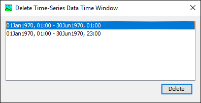
There are two ways to delete a time window. The first way is from the Time-Series Data Manager, accessed by clicking the Components menu and then selecting the Time-Series Data Manager command. Select the desired data type, then click on a time-series gage in the list; it will become highlighted. Press the Delete Window button to delete a time window. The Delete Time-Series Data Time Window window will open where you can select the window to delete (Figure 11). Click on the desired window and it will become highlighted. Press the Delete button to delete the highlighted time window. If you change your mind and do not want to delete a time window, press the X button in the upper corner of the Delete Time-Series Data Time Window window.
The second way to delete a time window is directly from the Watershed Explorer. Select a time window for a time-series gage; it will become highlighted. Keep the mouse over the time window icon and click the right mouse button. A context menu appears as shown in Figure 12; click the Delete Time Window command to delete the selected time window.

The user can change the start date, start time, end date, and end time of an existing time window. Use the Watershed Explorer to select the time window you wish to change. Click on the time window under the correct time-series component. The component will become the selected component and its data will be shown in the Component Editor as seen in Figure 13; the "Time Window" tab is automatically selected. Change the start date or other properties to the desired values. Click on a different tab in the Component Editor or elsewhere in the program interface to make the changes take affect.

Data Source
The data source determines how the data for a time-series component will be entered. There are three alternative methods for entering the data:
- The user may enter the time-series values by manually typing each one. A variation of this method is using the clipboard to copy and paste instead of manually typing. This first method is known as "Manual Entry."
- The user may load data into a Data Storage System (HEC-DSS) file. This method can be facilitated using the program HEC-DSSVue to create individual HEC-DSS files. The gage is linked to the time-series values stored in the file. This second method is known as "Single Record HEC-DSS."
- The user may store alternative versions of the time-series values in a HEC-DSS file. This method is used exclusively for forecasting operations with the Corps Water Management System (CWMS) and planning studies with the Watershed Analysis Tool (HEC-WAT). This third method is known as "Multiple Record HEC-DSS."
The selected data source will determine how the time-series values are entered. The values may be manually typed or linked to a HEC-DSS file. Compare Figure 14 and Figure 15 to see the differences in specifying the data sources.
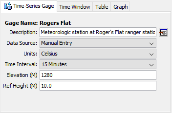
Figure 14. Component editor for a temperature gage with manually-entered data. Of the different data types, only temperature gages have elevation.
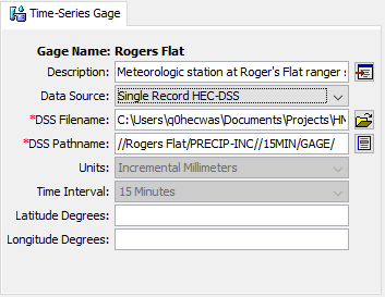
Figure 15. Component editor for a precipitation gage retrieving data from a Data Storage System (HEC-DSS) file. Of the different data types, only precipitation gages have latitude and longitude.
Data Units
The data units can only be selected for a manual entry time-series gage (Figure 14); they are retrieved automatically for both HEC-DSS options (Figure 15). Most types of time-series data have only two options for units; one for the system international unit system and one for the U.S. customary unit system. For example, discharge gages can use cubic meters per second (M3/S) or cubic feet per second (CFS). The precipitation time-series type has additional options for specifying incremental or cumulative data. The units available in the "Units" field will depend on the time-series type of the selected component. All time windows defined for a time-series component must use the same data units.
Generally you should choose the data units before entering any data for the gage. However, if you change the units after entering data, the data will be adjusted to the new units. There is no units conversion during the adjustment. The values are all kept the same but the assigned units are changed. This is helpful when the data is entered without first checking to make sure the data units are in the desired unit system.
Select the data units for a time-series gage using the Component Editor. Access the editor by selecting a time-series gage in the Watershed Explorer. The "Time-Series Gage" tab in the Component Editor will display the data units if the manual entry option is selected.
Time Interval
The time interval can only be selected for a manual entry time-series gage (Figure 14); it is retrieved automatically for both HEC-DSS options (Figure 15). An interval must be selected from the available choices that range from 1 minute to 1 day. All time windows defined for a time-series component must use the same time interval.
Generally, you should choose the time interval before entering any data for the component. However, if you change the time interval after entering data, the data will be adjusted to the new time interval. When the time interval is made shorter, the data for each time window will be adjusted so that it still begins at the start of the time window. The data will have the new, shorter time interval and there will be missing data from the last specified value to the end of the time window. When the time interval is made longer, the data for each time window will be adjusted so that it still begins at the start of the time window. The data will have the new, longer time interval and the end of the time window will be advanced so that no data is lost.
Select the time interval for a time-series gage using the Component Editor. Access the editor by selecting a time-series gage in the Watershed Explorer. The "Time-Series Gage" tab in the Component Editor will display the time interval if the manual entry option is selected.
Elevation
Certain atmospheric variables show a strong trend with elevation. Air pressure and air temperature both decrease as the elevation increases. Relative humidity increases as the elevation increases. The physics of water and air can be used to develop relationships for how these variables change with elevation. Therefore, calculating atmospheric variables at a location in the watershed requires both the elevation where the measurement was performed and the elevation where the variable should be calculated. The elevation must be entered for data types that require it. In general, the ground surface elevation (above sea level) at the measurement site is used. The value may be entered as either meters or feet, depending on the unit system of the gage. The requirements for entering elevation are shown in Table 1.
Reference Height
Some atmospheric variables change dramatically near the ground surface. Windspeed is very close to zero at the ground surface and increases as distance above the ground increases. Air temperature and relative humidity change significantly with distance above a snow covered surface. Therefore, calculating these atmospheric variables at the ground surface requires information about the height above the ground where the measurements were performed. While it is common for meteorologic instruments to be mounted on a tower 10 meters above the ground surface, other distances may be used at some installations. The instrument reference height must be entered for data types that require it. The value may be entered as either meters or feet, depending on the unit system of the gage. The requirements for entering reference height are shown in Table 1.
Latitude and Longitude
The most important atmospheric variable in hydrology is precipitation. Developing an accurate representation of a storm is critical to accurately simulating discharge throughout the watershed. Precipitation gages measure the rainfall at discrete locations within and adjacent to the watershed. Interpolation methods estimate precipitation continuously across the watershed based on the measured rainfall. The methods require a precise description of the location of each precipitation gage. The location is specified for each gage as the latitude and longitude. The latitude and longitude may be entered either as decimal degrees or as a triplet of degrees, minutes, and seconds. The method of entering the latitude and longitude is configured in the Program Settings. The requirements for entering latitude and longitude are shown in Table 1.
The degrees, minutes, and seconds are specified separately for the latitude and longitude. In general you should only specify the whole degrees and whole minutes. You can choose to specify whole or fractional seconds. If you enter more than 60 minutes or more than 60 seconds, the program will automatically adjust the degrees, minutes, or second as necessary to have 60 or fewer minutes and 60 or fewer seconds.
Table 1. Requirements for entering additional properties for gages.
Time-Series | Elevation | Reference Height | Latitude Longitude |
Precipitation | X | ||
Discharge | |||
Stage | |||
Temperature | X | X | |
Radiation | |||
Windspeed | X | ||
Air pressure | X | ||
Humidity | X | X | |
Altitude | |||
Crop Coefficient | |||
Snow Water Equivalent | |||
Sediment Load | |||
Concentration | |||
Percent | |||
Evapotranspiration | |||
Sunshine |
For example, if you entered 120 degrees and 64 minutes, the program would convert that data to 121 degrees and 4 minutes. A similar adjustment is made when the number of seconds is greater than 60. Alternately, you can specify the latitude and longitude in decimal degrees. In this case only the input for degrees is shown. Instead of entering a value such as 121 degrees, 4 minutes, and 17 seconds, a value in decimal degrees can be entered as 121.07139 degrees. Change the format for displaying and entering latitude and longitude in the program settings which are described earlier in Program Settings. The setting is found on the "General" tab.
General cartography conventions use negative longitude degrees in the Western hemisphere and positive longitude degrees in the Eastern hemisphere. Negative latitude degrees are used in the Southern hemisphere and positive latitude degrees are used in the Northern hemisphere. These conventions should be used for entry of latitude and longitude throughout the program.
Manual Entry
Manual entry is the simpliest way to get data values for a time-series gage. The values are manually typed for each date and time. All of the data should be reviewed after entry to verify accurate typing. If no value was recorded for a date and time, then the value should be left blank. The program does not automatically fill in missing data. Data recovery should be considered for extended periods of missing data.
Manual entry can also be used in combination with the clipboard to transfer data values from another computer program. Time-series values may be stored in a spreadsheet or other program. The values can be selected in the other program and copied to the clipboard. The values copied to the clipboard can be pasted in HEC-HMS. Using the clipboard can save a significant amount of manual typing and reduce errors when the time-series values are available in another program.
Manual entry time-series values are automatically stored in a HEC-DSS file in the project directory. The program uses the name of the gage to create a HEC-DSS file for storing the manual entry data. Manual entry values can be entered and then edited as many times as necessary to correct typing errors. Each time the data values are modified manually by the user, the data is automatically updated in the HEC-DSS file. One benefit of using a HEC-DSS file as an automatic storage solution is that the file can be reduced for other modeling projects.
Single Record HEC-DSS
Retrieving time-series data from a HEC-DSS file requires that the data be loaded in a file. The file can be stored on the local computer or on a network server. It is not a good idea to store the file on removable media since the file must be available whenever the time-series component is selected in the Watershed Explorer, and during simulations. Data for each gage can be stored in a separate file or one file can contain data for several gages. However, all data for a single time-series gage must be stored in the same HEC-DSS file and use appropriate pathname convention. It is best practice to store the HEC-DSS files holding gage data in the project directory, or a subdirectory of the project directory. The HEC-DSSVue utility (HEC 2003) can be used to load time-series data into a DSS file.
When the "Single Record HEC-DSS" option is selected, you must specify the filename to use for the time-series component (Figure 15). You may type the complete filename if you know it. To use a file browser to locate the file, press the Open File Chooser button to the right of the "DSS Filename" field. The browser allows you to find the desired file but it is limited to locating files with the DSS extension which is required for all Data Storage System files. Once you locate the desired file, click on it in the browser to select it and press the Select button. If you change your mind, press the Cancel button or the X button in the upper corner of the Select HEC-DSS File window to return to the Component Editor.
You must also specify the pathname to retrieve from the selected HEC-DSS file (Figure 15). You may type the complete pathname if you know it. Each pathname contains six parts called the A-part, B-part, C-part, D-part, E-part, and F-part. The pathname parts are separated with a slash and may contain spaces. The complete pathname, including slashes and spaces, can total up to 256 uppercase characters. The following is an example of an incremental precipitation pathname:
//COOPER SMITH DAM/PRECIP-INC/01OCT2001/15MIN/OBS/
Because of internal performance considerations, a HEC-DSS file will usually contain multiple records when storing long time-series. The different records will each have all the same pathname parts except for the D-part which indicates the starting time of each record. Any of the record pathnames can be selected and the program will automatically retrieve the correct data depending on the selected time window.
If you do not know the full pathname of the record you wish you use, you can use the pathname browser to specify it. You must select a HEC-DSS file first before the browser is available. Press the Select DSS Pathname button to the right of the "DSS Pathname" field to open the browser. The browser initially shows all of the records in the selected HEC-DSS file, organized by pathname in the selection table. You can scroll through the list and select a record pathname by clicking on it. Press the Select button at the bottom of the browser to choose that record and return to the Component Editor. If you change your mind and do not want to select a record pathname, press the Cancel button or the X button in the upper right of the Select Pathname From HEC-DSS File window. You can reduce the number of record pathnames shown in the selection table using the "Search by Parts" filters. A separate filter selection is shown for each of the six pathname parts. By selecting a choice for a filter, only pathnames that match that choice will be shown in the selection table. If you make choices in several filters, only pathnames that satisfy all of the choices will be shown in the selection table.
The program observes a very strict set of rules for data type and units within the record pathnames. Rules governing the C-part of the pathname are also enforced. Data cannot be used unless is follows the rules correctly; error messages will be generated if you attempt to use an invalid C-part, data type, or units. The acceptable data types for the different types of time-series data are shown in Table 2. The correct unit labels are shown in Table 3.
Table 2. Internal DSS data type label for different types of time-series data.
Time-Series | Type | Description |
Precipitation | PER-CUM | The incremental precipitation during each time interval. The C-part should be "PRECIP-INC". |
INST-CUM | The cumulative precipitation at the end of each interval. The C-part should be "PRECIP-CUM". | |
Discharge | PER-AVER | The average flow rate during each time interval, usually for time steps of 24 hours or longer. The C-part should be "FLOW". |
INST-VAL | The instantaneous flow rate at the end of each time interval. The C-part should be "FLOW". | |
Stage | PER-AVER | The average elevation during each interval, usually time steps of 24 hours or longer. The C-part should be "STAGE". |
INST-VAL | The instantaneous elevation at the end of each time interval. The C-part should be "STAGE". | |
Temperature | PER-AVER | The average temperature, in degrees, during each time interval. The C-part should be "TEMPERATURE". |
INST-VAL | The instantaneous temperature, in degrees, at the end of each time interval. The C-part should be "TEMPERATURE". | |
Radiation | PER-AVER | The average radiation, in power per area, occurring during each time interval. The C-part should be "RADIATION". |
| Windspeed | INST-VAL | The instantaneous windspeed at the end of each time interval. The C-part should be "WINDSPEED". |
| Air pressure | INST-VAL | The instantaneous air pressure at the end of each time interval. The C-part should be "PRESSURE". |
| Humidity | INST-VAL | The instantaneous humidity at the end of each time interval. The C-part should be "HUMIDITY". |
Altitude | INST-VAL | The instantaneous altitude at the end of each time interval. The C-part should be "ALTITUDE". |
| Crop Coefficient | INST-VAL | The instantaneous crop coefficient, as a dimensionless decimal number, occurring at the end of each time interval. The C-part should be "CROP COEFFICIENT". |
| Snow Water Equivalent | INST-VAL | The instantaneous snow water equivalent, as a depth at the end of each time interval. The C-part should be "SWE". |
| Sediment Load | PER-CUM | The total sediment load during each time interval. The C-part should be "LOAD". |
| Concentration | INST-VAL | The instantaneous concentration at the end of each time interval. The C-part should be "CONC". |
| Percent | INST-VAL | The instantaneous percent at the end of each time interval. The C-part should be "PERCENT". |
| Evapotranspiration | PER-CUM | The incremental evapo-transpiration during each time interval. The C-part should be "ET". |
| Sunshine | PER-AVER | The average sunshine during each time interval. The C-part should be "SUNSHINE HOURS". |
Table 3. Internal DSS units label for different types of time-series data.
Time-Series | Label | Description |
Precipitation | MM | Millimeters |
IN | Inches | |
Discharge | M3/S | Cubic meters per second |
CFS | Cubic feet per second | |
Stage | M | Meters |
FT | Feet | |
Temperature | DEG C | Degrees centigrade |
DEG F | Degrees Fahrenheit | |
Radiation | WATT/M2 | Watts per square meter |
LANG/MIN | Langleys per minute | |
Windspeed | KPH | Kilometers per hour |
M/S | Meters per second | |
MPH | Miles per hour | |
FT/S | Feet per second | |
Air Pressure | KPA | Kilo pascals |
IN HG | Inches of mercury | |
Humidity | % | Relative humidity |
Altitude | KM | Kilometers above sea level |
MILE | Miles above sea level | |
Crop Coefficient | UNSPECIF | Dimensionless coefficient |
Snow Water Equivalent | MM | Millimeters |
IN | Inches | |
Sediment Load | TONS | Tons |
TONNES | Metric tonnes | |
Concentration | MG/L | Milligrams per liter |
Percent | % | Percent |
Evapotranspiration | MM | Millimeters |
IN | Inches | |
Sunshine | HR | Hours |
Multiple Record HEC-DSS
The multiple record HEC-DSS data source is designed for forecasting operations with the Corps Water Management System (CWMS). The System provides forecasts of future conditions that are used to support operation decisions. It combines meteorologic and hydrologic data management with engineering simulation models. Meteorologic data includes radar-based precipitation measurements and gage measurements of atmospheric variables. Hydrologic data includes stage and discharge observations among others. Engineering models include hydrology, reservoir operations, hydraulics, and consequences. A typical forecast includes the following steps:
- Combine recently observed precipitation with forecast precipitation.
- Link the combined precipitation to HEC-HMS for computing channel flow.
- Transfer the flow to a reservoir model to determine the best operations for the dam.
- Connect the reservoir discharge to a hydraulic model to compute downstream flow.
- Map the downstream flow and estimate economic consequences, and in the case of severe flooding, the potential for life loss.
Forecast operations often consider more than one potential meteorologic forecast. The multiple meteorologic forecasts may result from alternative atmospheric models, atmospheric model ensemble members, or synthetic scenarios such as 150% of the forecast precipitation volume. The multiple record HEC-DSS data source is designed to facilitate the multiple hydrologic simulations necessary to evaluate each meteorologic alternative.
The multiple record data source includes a default selection for HEC-DSS file and pathname. The file and pathname are selected using the same steps already detailed for the Single Record HEC-DSS data source. The default selection will be used during simulations performed in HEC-HMS when it is not part of CWMS. However, when HEC-HMS is used with CWMS, the multiple record data source will be automatically switched to the correct meteorologic alternative based on the overall System configuration.
Table
The data for the current time window is shown in tabular form on the "Table" tab of the Component Editor (Figure 16). If you select a time-series gage in the Watershed Explorer, only the tab for the "Time-Series Gage" is shown in the Component Editor. If you select a time window under a time-series gage in the Watershed Explorer, the "Table" tab will be added to the Component Editor. Data in the table can be edited if the gage uses manual entry. Data is not editable if the gage retrieves data from a DSS file. Furthermore, if the gage uses DSS data and no time-series data is available for the specified time window, then the table will not contain any data.
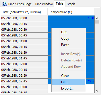
Figure 16. Manually entering data for a temperature gage. The fill command will be used to linearly interpolate between two known temperatures.
You can enter all of the data for each time window one value at a time in the table. However, there are tools to help you enter the data quickly. The table includes support for the clipboard. This means you can copy data stored in a spreadsheet or other file and then paste it into the table. You can also use the fill tool to enter or adjust data values in the table. Select the cells in the table you wish to fill and click the right mouse button. A context menu is displayed; select the Fill… command. The Fill Table Options window opens for you to control the process of filling and adjusting cell values. Options include interpolating the values between the first and last cell in the selection, several choices for interpolating and replacing missing values, copying the first selected cell value to all other selected cells, adding a constant value to all selected cells, and multiplying the selected cell values by a constant. Press the OK button to apply your choice, or the Cancel button to return to the table without making any changes.
Graph
The data for the current time window is shown in graphical form on the "Graph" tab of the Component Editor (Figure 17). If you select a time-series gage in the Watershed Explorer, only the tab for the "Time-Series Gage" is shown in the Component Editor. If you select a time window under a time-series gage in the Watershed Explorer, the "Graph" tab will be added to the Component Editor. Data in the graph cannot be edited regardless of whether the gage uses manual entry or retrieves data from a DSS file. If no time-series data is available for the specified time window, then the graph will not contain any data.
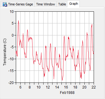
Figure 17. Viewing data for a discharge gage connected to a HEC-DSS file.