The outflow structures routing method is designed to model reservoirs with a number of uncontrolled outlet structures. For example, a reservoir may have a spillway and several low-level outlet pipes. While there is an option to include gates on spillways, the ability to control the gates is extremely limited at this time. There are currently no gates on outlet pipes. However, there is an ability to include a time-series of releases in addition to the uncontrolled releases from the various structures. An external analysis may be used to develop the additional releases based on an operations plan for the reservoir.

Additional features in the reservoir for culverts and pumps allow the simulation of interior ponds. This class of reservoir often appears in urban flood protection systems. A small urban creek drains to a collection pond adjacent to a levee where flood waters collect. When the main channel stage is low, water in the collection pond can drain through culverts into the main channel. Water must be pumped over the levee when the main channel stage is high.

Storage Method

There are two different options for specifying the storage relationship. The first option is the Elevation-Storage choice, as shown in Figure 1. The user must select an elevation-storage curve from the available curves in the Paired Data Manager. After the routing is complete, the program will compute the elevation and storage for each time interval. The second option is the Elevation-Area choice, which requires the selection of an elevation-area curve from the available curves in the Paired Data Manager. With this choice, the program automatically transforms the elevation-area curve into an elevation-storage curve using the conic formula. After the routing is complete, the program will compute the elevation, surface area, and storage for each time interval.

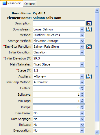
Figure 1. Reservoir component editor using the outflow structures routing method with three outlets, one spillway, and one dam top representing an emergency spillway.

You must select an appropriate function to define the selected storage method. For example, if you select the Elevation-Storage method you must select an appropriate elevation-storage paired data function that defines the storage characteristics of the reservoir. The appropriate selection list will be shown directly under the storage method selection list. Any necessary paired data functions must be defined in the paired data manager before they can be used in the reservoir. Choose an appropriate function in each selection list. If you wish, you can use a chooser by clicking the paired data button next to the selection list. A chooser will open that shows all of the paired data functions of that type. Click on a function to view its description.

Initial Condition

The initial condition sets the amount of storage in the reservoir at the beginning of a simulation. Therefore, the simplest option is to specify the Storage as a volume of water in the reservoir. For convenience, other options are also provided. The Inflow=Outflow method takes the inflow to the reservoir at the beginning of the simulation, and determines the pool elevation necessary to cause that outflow through the outlet structures. The pool elevation is then used in the elevation-storage curve to determine the matching storage. The pool Elevation method can also be selected for the initial condition. In this case, the elevation provided by the user is used to interpolate a storage value from the elevation-storage curve. The initial condition options depend on the selected storage method and are shown in Table 1.

Table 1. Available initial condition options for different storage methods used with the outlet structures routing method.

Tailwater Method

The selected tailwater method determines how submergence will be calculated for the individual structures specified as part of the reservoir. When a structure is submerged, the discharge through the structure will decrease in accordance with the physics of the structure and the tailwater elevation for each time interval. Only one tailwater method can be selected and it is applied to all structures specified as part of the reservoir.

The Assume None method is used in cases where reservoir tailwater has no affect on the reservoir outflow.

The Reservoir Main Discharge method is typically used with reservoirs that span the stream channel and are not influenced by backwater from downstream sources. For such cases, the tailwater below the reservoir only comes from the reservoir releases. A rating curve defined by an elevation-discharge paired data function must be selected to convert reservoir outflow to stage. The elevation-discharge function must be defined before it can be used in the reservoir. Choose an appropriate function in the selection list or use a chooser by clicking the paired data button next to the selection list. The rating curve should be specified in the same vertical datum as the function used to describe the storage characteristics of the reservoir.

The Downstream Of Main Discharge method is typically used with reservoirs that represent an interior pond or pump station, and the outflow from the reservoir will be a significant impact on the downstream stage. In this case, the outflow from the reservoir is combined with all other inflows to the element downstream of the reservoir. That combined inflow is used in combination with a rating curve to determine the stage for the reservoir tailwater. The elevation-discharge function for the rating curve must be defined in the paired data manager before it can be used in the reservoir. Choose an appropriate function in the selection list or use a chooser by clicking the paired data button next to the selection list. The rating curve should be specified in the same vertical datum as the function used to describe the storage characteristics of the reservoir.

The Specified Stage method is typically used with reservoirs that represent an interior pond or pump station, and the outflow from the reservoir will have minimal affect on the downstream stage. In this case, the outflow from the reservoir is adjusted for submergence based on the stage specified in a stage time-series gage. The gage must be defined in the time-series data manager before it can be used in the reservoir. Choose an appropriate gage in the selection list or use a chooser by clicking the gage data button next to the selection list. The stage should be specified in the same vertical datum as the function used to describe the storage characteristics of the reservoir.

The Fixed Stage method is typically used with reservoirs that represent an interior pond or pump station. The same stage is used for all time intervals in a simulation. In this case, the outflow from the reservoir is adjusted for submergence based on the specified stage.

Auxiliary Discharge Location

All reservoirs have a primary discharge to the downstream. Flow through outlets, spillways, and other structures leaves the reservoir and enters some type of channel. However, some reservoirs also have an auxiliary discharge in addition to the primary discharge. The flow exiting through the auxiliary discharge location does not enter the same channel as the main discharge. The auxiliary discharge may be an emergency spillway that enters a secondary channel that eventually enters the main downstream channel. The auxiliary discharge could also be a withdrawal for urban consumptive use or possibly an agricultural irrigation canal.

Each structure added to the reservoir can be designated to discharge to the Main or Auxiliary direction. The default is for a structure to discharge in the main direction. Optionally, one or more outlet structures can be set to discharge in the auxiliary direction. Both the main and auxiliary locations use separate tailwater methods. An appropriate tailwater selection should be made for the auxiliary location if it will be used. The selection of tailwater method is independent for the two directions so they may be the same or different. When a rating curve is used for the tailwater method, the rating curve should be appropriate for the main or auxiliary location where it is selected for use.

Time Step Control

The Outflow Structures routing method uses an adaptive time step algorithm. The time step specified in the Control Specifications is used during periods of a simulation when the reservoir pool elevation is changing slowly. However, under conditions when the pool elevation is changing rapidly, such as during a dam break, a shorter time step is used. The adaptive time step algorithm automatically selects an interval based on the rates at which the pool elevation, storage, and outflow are changing. Results are always computed at the time interval specified in the Control Specifications. Any adaptive steps taken between these time intervals are used internally to obtain the solution but are not stored for later use or display. The adaptive time step algorithm obtains very good solutions of the pool elevation and outflow. However, many more calculations may be necessary to obtain the results. For preliminary simulations, especially those with a long time window, it may be advantageous to disable the adaptive time step portion of the algorithm. This can be accomplished in the reservoir component editor (Figure 1) by selecting the Simulation Interval time step method. Simulations with a short time window or final simulations with a long time window should use the Automatic Adaption time step method to get the best possible precision in the results.

Outlets

Outlets can only be included in reservoirs using the Outflow Structures routing method. Outlets typically represent structures near the bottom of the dam that allow water to exit in a controlled manner. They are often called gravity outlets because they can only move water when the head in the reservoir is greater than the head in the tailwater. Up to 10 independent outlets can be included in the reservoir. Select the number of outlets you wish to include. An icon for each outlet will be added to the reservoir icon in the Watershed Explorer. You will need to click on the individual outlet icon to enter parameter data for it. There are two different methods for computing outflow through an outlet: culvert or orifice.

Culvert Outlet

The culvert outlet allows for partially full or submerged flow through a culvert with a variety of cross-sectional shapes. It can account for inlet controlled outflow or outlet control. A typical culvert outlet is shown in Figure 2.

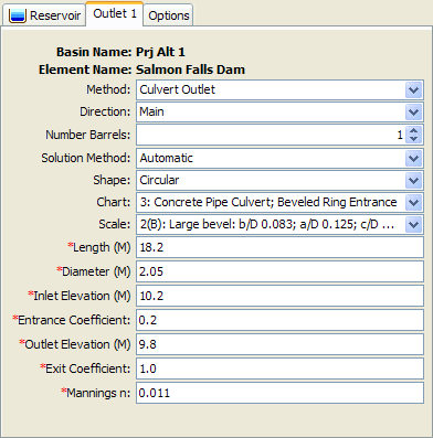
Figure 2. Outlet editor with the culvert method selected.

You must select a solution method for the culvert: inlet control, outlet control, or automatic. You may select Inlet Control if it is known that at all times during a simulation the culvert outflow will be controlled by a high pool elevation in the reservoir. You may likewise select Outlet Control if it is known that at all times the culvert outflow will be controlled by a high tailwater condition. In general, it is best to select Automatic control and the program will automatically determine the controlling inlet or outlet condition.

You must select the number of identical barrels. This can be used to specify several culvert outlets that are identical in all parameters. There can be up to 10 identical barrels.

The shape specifies the cross-sectional shape of the culvert: circular, semi circular, elliptical, arch, high-profile arch, low-profile arch, pipe arch, box, or con span. The shape you choose will determine some of the remaining parameters in the Component Editor. The parameters you will need to enter are shown in Figure 2.

The chart specifies the FHWA chart identification number. Only the charts that apply to the selected shape will be shown in the selection list (Figure 2).

The scale specifies the FHWA scale identification number. Only the scales that apply to the selected chart number will be shown in the selection list.

Table 2. Listing of which parameters are required for each cross section shape.

The length of the culvert must be specified. This should be the overall length of the culvert including any projection at the inlet or outlet.

The inlet elevation must be specified as the invert elevation at the bottom of the culvert on the inlet side. The inlet side is always assumed to be in the reservoir pool. This should be measured in the same vertical datum as the paired data functions defining the storage characteristics of the reservoir.

The entrance coefficient describes the energy loss as water moves into the inlet of the culvert. Values may range from 0.2 up to 1.0.

The exit coefficient describes the energy loss that occurs when water expands as it leaves the culvert outlet. Typically the value is 1.0.

The outlet elevation must be specified as the invert elevation at the bottom of the culvert on the outlet side. The outlet side is always assumed to be in the reservoir tailwater. This should be measured in the same vertical datum as the paired data functions defining the storage characteristics of the reservoir.

A Manning's n value should be entered that describes the roughness in the culvert. At this time, the same n value must be used for the entire length of the culvert, as well as the entire top, sides, and bottom.

Orifice Outlet

The orifice outlet assumes sufficient submergence on the outlet for orifice flow conditions to dominate. It should not be used to represent an outlet that may flow only partially full. The inlet of the structure should be submerged at all times by a depth at least 0.2 times the diameter. A typical orifice outlet editor is shown in Figure 3.

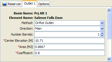
Figure 3. Outlet editor with the orifice method selected.

You must select the number of identical barrels. This can be used to specify several culvert outlets that are identical in all parameters. There can be up to 10 identical barrels.

The center elevation specifies the center of the cross-sectional flow area. This should be measured in the same vertical datum as the paired data functions defining the storage characteristics of the reservoir. It is used to compute the head on the outlet, so no flow will be released until the reservoir pool elevation is above this specified elevation.

The cross-sectional flow area of the outlet must be specified. The orifice assumptions are independent of the shape of the flow area.

The dimensionless discharge coefficient must be entered. This parameter describes the energy loss as water exits the reservoir through the outlet.

Spillways

Spillways can only be included in reservoirs using the Outflow Structures routing method. Spillways typically represent structures at the top of the dam that allow water to go over the dam top in a controlled manner. Up to 10 independent spillways can be included in the reservoir. Select the number of spillways you wish to include. An icon for each spillway will be added to the reservoir icon in the Watershed Explorer. You will need to click on the individual outlet icon to enter parameter data for it. There are three different methods for computing outflow through a spillway: broad-crested, ogee, and user specified. The broad-crested and ogee methods may optionally include gates. If no gates are selected, then flow over the spillway is unrestricted. When gates are included, the flow over the spillway will be controlled by the gates. Up to 10 independent gates may be included on a spillway.

Broad-Crested Spillway

The broad-crested spillway allows for controlled flow over the top of the reservoir according to the weir flow assumptions. A typical broad-crested spillway editor is shown in Figure 4.

The crest elevation of the spillway must be specified. This should be measured in the same vertical datum as the paired data functions defining the storage characteristics of the reservoir.

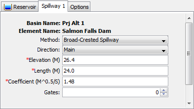
Figure 4. Spillway editor with the broad-crested method selected.

The length of the spillway must be specified. This should be the total width through which water passes.

The discharge coefficient accounts for energy losses as water enters the spillway, flows through the spillway, and eventually exits the spillway. Depending on the exact shape of the spillway, typical values range from 1.10 to 1.66 in System International units (2.0 to 3.0 US Customary units).

Ogee Spillway

The ogee spillway allows for controlled flow over the top of the reservoir according to the weir flow assumptions. However, the discharge coefficient in the weir flow equation is automatically adjusted when the upstream energy head is above or below the design head. A typical ogee spillway editor is shown in Figure 5.

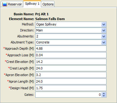
Figure 5. Spillway editor with the ogee method selected.

The ogee spillway may be specified with concrete or earthen abutments. These abutments should be the dominant material at the sides of the spillway above the crest. The selected material is used to adjust energy loss as water passes through the spillway. The spillway may have one, two, or no abutments depending on how the spillway or spillways in a reservoir are conceptually represented.

The ogee spillway is assumed to have an approach channel that moves water from the main reservoir to the spillway. If there is such an approach channel, you must specify the depth of the channel, and the energy loss that occurs between the main reservoir and the spillway. If there is no approach channel, the depth should be the difference between the spillway crest and the bottom of the reservoir, and the loss should be zero.

The crest elevation of the spillway must be entered. This should be measured in the same vertical datum as the paired data functions defining the storage characteristics of the reservoir.

The crest length of the spillway must be specified. This should be the total width through which water passes.

The apron elevation is the elevation at the bottom of the ogee spillway structure. This should be measured in the same vertical datum as the paired data functions defining the storage characteristics of the reservoir.

The apron width must be specified. This should be the total width of the spillway bottom.

The design head is the total energy head for which the spillway is designed. The discharge coefficient will be automatically calculated when the head on the spillway departs from the design head.

Specified Spillway

The user-specified spillway can be used to represent spillways with flow characteristics that cannot be represented by the broad-crested or ogee weir assumptions. The user must create an elevation-discharge curve that represents the spillway discharge as a function of reservoir pool elevation. At this time there is no ability to include submergence effects on the spillway discharge. Therefore the user-specified spillway method should only be used for reservoirs where the downstream tailwater stage cannot affect the discharge over the spillway. A typical user-specified spillway editor is shown in Figure 6.

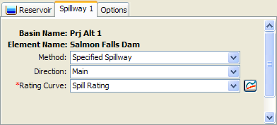
Figure 6. Spillway editor with the user-specified method selected.

The rating curve describing flow over the spillway must be selected. Before it can be selected it must be created in the Paired Data Manager as an elevation-discharge function. The function must be calculated external to the program on the basis of advanced spillway hydraulics or experimentation.

Spillway Gates

Spillway gates are an optional part of specifying the configuration of a spillway. They may be included on either broad-crested or ogee spillways. The number of gates to use for a spillway is specified on the spillway editor (Figure 4 and Figure 5). An icon for each gate will be added to the spillway icon under the reservoir icon in the Watershed Explorer. You will need to click on the individual gate icon to enter parameter data for it. There are two different methods for computing outflow through a gated spillway: sluice or radial. In both cases you may specify the number of identical units; each identical unit has exactly the same parameters, including how the gate is controlled.

Sluice Gate

A sluice gate moves up and down in a vertical plane above the spillway in order to control flow. The water passes under the gate as it moves over the spillway. For this reason it is also called a vertical gate or underflow gate. The editor is shown in Figure 7.

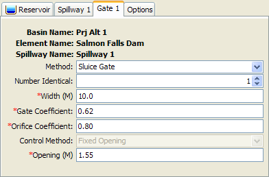
Figure 7. Sluice gate editor for spillways.

The width of the sluice gate must be specified. It should be specified as the total width of an individual gate.

The gate coefficient describes the energy losses as water passes under the gate. Typical values are between 0.5 and 0.7 depending on the exact geometry and configuration of the gate.

The orifice coefficient describes the energy losses as water passes under the gate and the tailwater of the gate is sufficiently submerged. A typical value for the coefficient is 0.8.

Radial Gate

A radial gate rotates above the spillway with water passing under the gate as it moves over the spillway. This type of gate is also known as a tainter gate. The editor is shown in Figure 8.

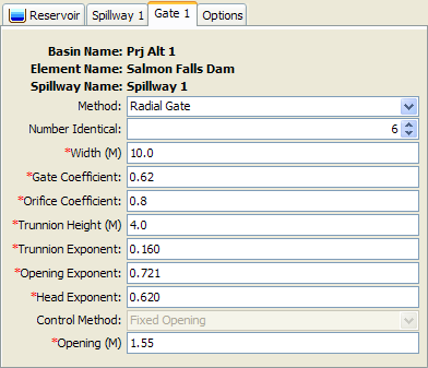
Figure 8. Radial gate editor for spillways.

The width of the radial gate must be specified. It should be specified as the total width of an individual gate.

The gate coefficient describes the energy losses as water passes under the gate. Typical values are between 0.5 and 0.7 depending on the exact geometry and configuration of the gate.

The orifice coefficient describes the energy losses as water passes under the gate and the tailwater of the gate is sufficiently submerged. A typical value for the coefficient is 0.8.

The pivot point for the radial gate is known as the trunnion. The height of the trunnion above the spillway must be entered.

The trunnion exponent is part of the specification of the geometry of the radial gate. A typical value is 0.16.

The gate opening exponent is used in the calculation of flow under the gate. A typical value is 0.72.

The head exponent is used in computing the total head on the radial gate. A typical value is 0.62.

Controlling Spillway Gates

An important part of defining gates on a spillway is the specification of how each gate will operate. It is rare that a gate is simply opened a certain amount and then never changed. Usually gates are changed on a regular basis in order to maintain the storage in the reservoir pool at targets; usually seasonal targets will be defined in the reservoir regulation manual. Under some circumstances, the gate operation may be changed to prevent flooding or accommodate other special concerns. At this time there is only one method for controlling spillway gates but additional methods will be added in the future.

The Fixed Opening control method only accommodates a single setting for the gate. The distance between the spillway and the bottom of the gate is specified. The same setting is used for the entire simulation time window.

Dam Tops

Dam tops can only be included in reservoirs using the Outflow Structures routing method. These typically represent the top of the dam, above any spillways, where water goes over the dam top in an uncontrolled manner. In some cases it may represent an emergency spillway. Up to 10 independent dam tops can be included in the reservoir. Select the number of dam tops you wish to include. An icon for each dam top will be added to the reservoir icon in the Watershed Explorer. You will need to click on the individual dam top icon to enter parameter data for it. There are two different methods for computing outflow through a dam top: level or non-level.

Level Dam Top

The level dam top assumes flow over the dam can be represented as a broad-crested weir. The calculations are essentially the same as for a broad-crested spillway. They are included separately mostly for conceptual representation of the reservoir structures. A typical level dam top is shown in Figure 9.

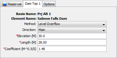
Figure 9. Dam top editor with the level overflow method selected.

The crest elevation of the dam top must be specified. This should be measured in the same vertical datum as the paired data functions defining the storage characteristics of the reservoir.

The length of the dam top must be specified. This should be the total width through which water passes, excluding any amount occupied by spillways if any are included.

The discharge coefficient accounts for energy losses as water approaches the dam top and flows over the dam. Depending on the exact shape of the dam top, typical values range from 1.10 to 1.66 in System International units (2.0 to 3.0 US Customary units).

Non-Level Dam Top

The non-level dam top assumes that the top of the dam can be well-represented by a cross section with eight station-elevation pairs. A separate flow calculation is carried out for each segment of the cross section. The broad-crested weir assumptions are made for each segment. A typical non-level dam top is shown in Figure 10.

A cross section must be selected which describes the shape of the top of the dam with a simplified eight point shape. From abutment to abutment of the dam, but should not include any spillways that may be included. It may be necessary to use multiple dam tops to represent the different sections of the dam top between spillways. The cross section should extend from the dam top up to the maximum water surface elevation that will be encountered during a simulation. The cross section must be defined in the paired data manager before it can be used in the reservoir element.

The discharge coefficient accounts for energy losses as water approaches the dam top and flows over the dam. The same value is used for all segments of the dam top. Typical values range from 2.6 to 4.0 depending on the exact shape of the dam top.

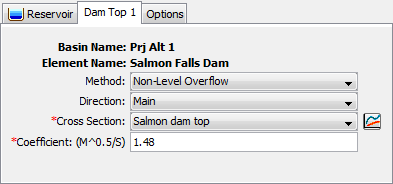
Figure 10. Dam top editor with the non-level overflow method selected.

Pumps

Pumps can only be included in reservoirs using the Outflow Structures routing method. These typically represent pumps in interior ponds or pump stations that are intended to move water out of the reservoir and into the tailwater when gravity outlets alone cannot move sufficient water. Up to 10 independent pumps can be included in the reservoir. Select the number of pumps you wish to include. An icon for each pump will be added to the reservoir icon in the Watershed Explorer. You will need to click on the individual pump icon to enter parameter data for it. There is only one method for computing outflow through a pump: head-discharge pump.

Head-Discharge Pump

The head-discharge pump is designed to represent low-head, high-flow situations. This means that the pump is designed for high flow rates against a relatively small head. The pump can be controlled to come on and shut off as the reservoir pool elevation changes. A typical head-discharge pump is shown in Figure 11.

The number of identical units must be specified. This allows data to be entered only once when there are multiple pump units with exactly the same parameters.

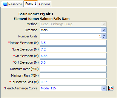
Figure 11. Pump editor with the head-discharge method selected.

The intake elevation defines the elevation in the reservoir pool where the pump takes in water. This should be measured in the same vertical datum as the paired data functions defining the storage characteristics of the reservoir.

The line elevation defines the highest elevation in the pressure line from the pump to the discharge point. This should be measured in the same vertical datum as the paired data functions defining the storage characteristics of the reservoir.

You must specify the elevation when the pump turns on. This should be measured in the same vertical datum as the paired data functions defining the storage characteristics of the reservoir. Once the pump turns on, it will remain on until the reservoir pool elevation drops below the trigger elevation to turn the pump off.

You must specify the elevation when the pump turns off. This should be measured in the same vertical datum as the paired data functions defining the storage characteristics of the reservoir. This elevation must be lower than the elevation at which the pump turns on.

The specification of a minimum rest time is optional. If it is used, once a pump shuts off it must remain off the specified minimum rest time even if the reservoir pool elevation reaches the trigger elevation to turn the pump on.

The specification of a minimum run time is optional. If it is used, once a pump turns on it must remain on the specified minimum run time even if the reservoir pool elevation drops below the trigger elevation to turn the pump off. The only exception is if the pool elevation drops below the intake elevation, then the pump will shut off even though the minimum run time is not satisfied.

The equipment loss includes all energy losses between the intake and discharge points, including the pump itself. This loss is added to the head difference due to reservoir pool elevation and tailwater elevation to determine the total energy against which the pump must operate.
The head-discharge curve describes the capacity of the pump as a function of the total head. Total head is the head difference due to reservoir pool elevation and tailwater elevation, plus equipment loss. A curve must be defined as an elevation-discharge function in the paired data manager before it can be selected for a pump in the reservoir. You can press the paired data button next to the selection list to use a chooser. The chooser shows all of the available elevation-discharge functions in the project. Click on a function to view its description.

Dam Break

Dam break can only be included in reservoirs using the Outflow Structures routing method. Only one dam break can be included in the reservoir. Choose whether you wish to include dam break. An icon for the dam break will be added to the reservoir icon in the Watershed Explorer. You will need to click on the dam break icon to enter parameter data for it. There are two different methods for computing outflow through a dam break: overtop and piping.

Overtop Dam Break

The overtop dam break (Figure 12) is designed to represent failures caused by overtopping of the dam. These failures are most common in earthen dams but may also occur in concrete arch, concrete gravity, or roller compacted dams as well. The failure begins when appreciable amounts of water begin flowing over or around the dam face. The flowing water will begin to erode the face of the dam. Once erosion begins it is almost impossible to stop the dam from failing. The method begins the failure at a point on the top of the dam and expands it in a trapezoidal shape until it reaches the maximum size. Flow through the expanding breach is modeled as weir flow.

The top elevation is the top of the dam face. The breach may be initiated at a lower elevation than the top depending on the selection of the trigger. This information is used to constrain the top of the breach opening as it grows. It should be measured in the same vertical datum as the paired data functions defining the storage characteristics of the reservoir.

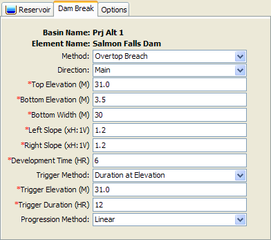
Figure 12. Dam break editor with the overtop breach method selected.

The bottom elevation defines the elevation of the bottom of the trapezoidal opening in the dam face when the breach is fully developed. This should be measured in the same vertical datum as the paired data functions defining the storage characteristics of the reservoir.

The bottom width defines the width of the bottom of the trapezoidal opening in the dam face when the breach is fully developed.

The left side slope is dimensionless and entered as the units of horizontal distance per one unit of vertical distance. The right side slope is likewise dimensionless and entered as the units of horizontal distance per one unit of vertical distance.

The development time defines the total time for the breach to form, from initiation to reaching the maximum breach size. It should be specified in hours.

There are three methods for triggering the initiation of the failure: elevation, duration at elevation, and specific time. Depending on the method you choose, additional parameters will be required. For the Elevation method, you will enter an elevation when the failure should start. The breach will begin forming as soon as the reservoir pool elevation reaches that specified elevation. For the Duration at Elevation method, you will enter an elevation and duration to define when the failure should start. The reservoir pool will have to remain at or above the specified elevation for the specified duration before the failure will begin. For the Specific Time method, the breach will begin opening at the specified time regardless of the reservoir pool elevation. When specifying an elevation, it should be measured in the same vertical datum as the paired data functions defining the storage characteristics of the reservoir.

The progression method determines how the breach grows from initiation to maximum size during the development time. Select the Linear method to have the breach grow in equal increments of depth and width. Select the Sine Wave method to have the breach grow quickly in the early part of breach development and more slowly as it reaches maximum size. The speed varies according to the first quarter cycle of a since wave. Select the User Curve method to have the breach grow according to a specified pattern. You will need to select a curve in the selection list, which will show all percentage curves defined in the paired data manager. The independent variable should range from 0 to 100 percent and define the percentage of the development time. The dependent variable should define the percentage opening of the maximum breach size. The function must be monotonically increasing.

Piping Dam Break

The piping dam break is designed to represent failures caused by piping inside the dam. These failures typically occur only in earthen dams. The failure begins when water naturally seeping through the dam core increases in velocity and quantity enough to begin eroding fine sediments out of the soil matrix. If enough material erodes, a direct piping connect may be established from the reservoir water to the dam face. Once such a piping connect is formed it is almost impossible to stop the dam from failing. The method begins the failure at a point in the dam face and expands it as a circular opening. When the opening reaches the top of the dam, it continues expanding as a trapezoidal shape. Flow through the circular opening is modeled as orifice flow while in the second stage it is modeled as weir flow.

The piping dam break (Figure 13) uses many of the same parameters as the overtop dam break. The top elevation, bottom elevation, bottom width, left slope, and right slope all are used to describe a trapezoidal breach opening that will be the maximum opening in the dam. These are only used once the piping opening transitions to an open breach. The parameters for development time, trigger method, and progression method are also the same for defining when the failure initiates, how long it takes to attain maximum breach opening, and how the breach develops during the development time. The remaining parameters, unique to piping dam break, are described below.

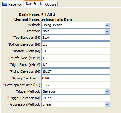
Figure 13. Dam break editor with the piping breach method selected.

The piping elevation indicates the point in the dam where the piping failure first begins to form. This should be measured in the same vertical datum as the paired data functions defining the storage characteristics of the reservoir.

The piping coefficient is used to model flow through the piping opening as orifice flow. As such, the coefficient represents energy losses as water moves through the opening.

Dam Seepage

Dam seepage can only be included in reservoirs using the Outflow Structures routing method. Most dams have some water seeping through the face of the dam. The amount of seepage depends on the elevation of water in the dam, the elevation of water in the tailwater, the integrity of the dam itself, and possibly other factors. In some situations, seepage from the pool through the dam and into the tailwater can be a significant source of discharge that must be modeled. Interior ponds may discharge seepage water but in some situations water in the main channel may seep through the levee or dam face and enter the pool. Both of these situations can be represented using the dam seepage structure.

There can only be one dam seepage structure in a reservoir that must represent all sources and sinks of seepage. When water seeps out of the reservoir, the seepage is automatically taken from the reservoir storage and added to the main tailwater discharge location. This is the mode of seepage when the pool elevation is greater than the tailwater elevation. Seepage into the reservoir happens when the tailwater elevation is higher than the pool elevation. In this mode the appropriate amount of seepage is added to reservoir storage, but it is not subtracted from the tailwater.

Tabular Seepage

The tabular seepage method uses an elevation-discharge curve to represent seepage as shown in Figure 14. Usually the elevation-discharge data will be developed through a geotechnical investigation separate from the hydrologic study. A curve may be specified for inflow seepage from the tailwater toward the pool, and a separate curve selected for outflow seepage from the pool to the tailwater. The same curve may be selected for both directions if appropriate. Any curve used for dam seepage must first be created in the Paired Data Manager. If a curve is not selected for one of the seepage directions, then no seepage will be calculated in that direction.

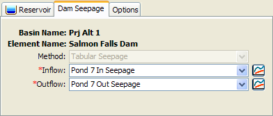
Figure 14. Dam seepage editor showing seepage into a reservoir.

Additional Release

An additional release can only be included in reservoirs using the Outflow Structures routing method. In most situations a dam can be properly configured using various outlet structures such as spillways, outlets, etc. The total outflow from the reservoir can be calculated automatically using the physical properties entered for each of the included structures. However, some reservoirs may have an additional release beyond what is represented by the various physical structures. In many cases this additional release is a schedule of managed releases achieved by operating spillway gates. The additional release can be used in combination with other outlet structures to determine the total release from the reservoir.

The additional release that will be specified must be stored as a discharge gage. The appropriate gage can be selected in the editor as shown in Figure 15. The gage must be defined in the Time-Series Data Manager before it can be selected. You can press the time-series data button next to the selection list to use a chooser. The chooser shows all of the available discharge gages in the project. Click on a gage to view its description.

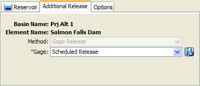
Figure 15. Additional release editor showing a selected discharge gage.

Evaporation

Evaporation can only be included in reservoirs using the Outflow Structures routing method. Additionally, the reservoir must be set to use the elevation-area storage option. Water losses due to evaporation may be an important part of the water balance for a reservoir, especially in dry or desert environments. The evaporation losses are different from other structures because they do not contribute to either main or auxiliary outflow. They are accounted separately and available for review with the other time-series results for the reservoir. An evaporation depth is computed for each time interval and then multiplied by the current surface area.

Monthly Evaporation

The monthly evaporation method can be used to specify a separate evaporation rate for each month of the year, entered as a total

depth for the month. The evaporation data must be developed through separate, external analysis and entered as shown in Figure 16.

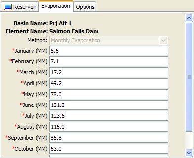
Figure 16. Evaporation editor showing the monthly evaporation method for a reservoir.