Download PDF
Download page Hyetograph Surface Creation Tool.
Hyetograph Surface Creation Tool
TIN disaggregation is the process of taking a single TIN in conjunction with temporal controls to generate a series of shorter timespan TINs that have the same aggregate total as the original TIN and also incorporate the temporal information from the given temporal controls. The temporal controls may be either one or more georeferenced hyetographs or a temporal pattern. When multiple hyetographs are used, the temporal pattern differs within the TIN based on the location of any particular location in the TIN with respect to the locations of the supplied hyetographs.
One example of where TIN disaggregation is useful is in the modeling of historical storms where no radar information is available. It is not unusual for storm hyetographs to have durations of 15 minutes, 1 hour, 6 hours and 24 hours for a single event. Some hyetographs may even be irregular interval time series, recording the time and date when each .01 inches of rainfall accumulate. A storm total TIN is simple to generate using all the data available (refer to the TriangulateTin command line utility). What if a series of 1-hour TINs is required? The 15 minute and 1 hour hyetograph data would be simple to utilize but to incorporate the longer time span data becomes a bigger challenge. In addition, the 24 hour reports may be a combination of midnight to midnight, 7am-7am, or 8am-8am readings. Using all the available data and attempting to accomplish this process manually can be a very time consuming task. By creating a single aggregate TIN representing the storm total and then using the more resolute reports for temporal distribution, a series of short duration TINs can be created which can then be used to generate subbasin average hyetographs or projected onto a set of gridded TINs for use by other programs.
Although the disaggregation technique processes a single TIN to create the shorter duration TINs, it can be inconvenient to specify a single TIN for perhaps a 24-hour timespan, load another TIN for the following day, and repeat the disaggregation process for a precipitation event that covers several days or weeks. Processing the entire storm as a single aggregate is not feasible in this situation because it would not respect the boundary conditions of the discrete TINs, allowing the temporal pattern for the entire timespan to possibly shift precipitation from one discrete TIN timespan to another if there was some variance between the distribution for the hyetographs and the TINs. HEC-MetVue allows the aggregate TIN that is referenced to be optionally processed by applying the disaggregation process independently to each TIN that comprises the aggregate TIN. When operating in this fashion, each TIN is independently disaggregated. In addition, the set of shorter duration TINs that are created will have exactly the same aggregate total as the original individual discrete TINs from which they were created, while at the same time creating a set of TINs that span the entire aggregate TIN timespan.
Several options are available for creating the resultant TIN datasets. As mentioned above, one or more hyetographs or a temporal pattern can be used. The hyetographs can be georeferenced by using a combination of DSS record metadata and name matching or a GageInterp control file, as specified in the GageInterp User's Manual (HEC, 2016). The hyetograph based TIN disaggregation tool  is available on the main HEC-MetVue tool bar and it provides access to the editor. A description of the features available in the editor are provided in the tables below.

Item | Description |
1 | This option is used to process the aggregate TIN as a single surface and disregard any discrete TINs that were used to create it. |
2 | This option is used to process the discrete TINs that the aggregate is comprised of one at a time as described above. When this option is selected, the ability to override the timespans as described in item 3 and the option to specify a temporal pattern are both disabled. When processing each discrete TIN the program uses the actual timespan information associated with the selected TINs. |
3 | This can be used to modify the starting and ending date of the aggregate TIN. |
4 | This is the methodology to use to define the temporal pattern. Depending on the option selected, certain portions of the remainder of the dialog will differ. The name matching option shown here allows the use of a combination of methods to georeference the list of hyetographs. |
5 | Hyetographs need to be georeferenced to be used. Knowing the longitude and latitude is essential. The program supports three options for defining the location as shown in items 6-8 below. |
6 | Use DSS path metadata. DSS supports storing the longitude and latitude in the time series records. One caution: every DSS path must hold its own metadata and a storm may cross multiple time series records in the data store. |
7 | Use a shapefile with hyetograph locations. This shapefile must be a POINT type of shapefile and a NAME, ID, or DSSB column must be present within the .DBF file. |
8 | Use aggregate TIN for hyetograph locations. If the aggregate TIN was constructed using the hyetographs/gages specified the process can match the name to the DSS B pathname part. Note that if the aggregate image is a radar image or some other image not based on the original hyetographs directly, this option will not resolve anything. |
9 | This gives a listing of the hyetograph paths and the DSS file they reside in that will be used for the analysis. Note that if there are any hyetographs that are specified that cannot be georeferenced, the process will fail. |
10 | This button will bring up a dialog (the same dialog used by DSSVue) to select hyetographs to use for the temporal distribution. |
11 | This button will clear the list of hyetographs used for temporal distribution. |
12 | This button will remove the highlighted hyetographs from the list of hyetographs used for temporal distribution. |
13 | This defines the geographic extent of the resultant images. The georeferenced hyetographs are converted to a resultant TIN (this TIN can vary over time if there is missing data) and this forms the basis for the boundary of valid data if the option to have the hyetographs define the boundary is used. If the aggregate image defines the extent, points on the aggregate image that fall outside the perimeter of the hyetograph generated TIN(s) use a weighted extrapolation technique of nearby hyetograph TIN locations to determine the temporal distribution. |
14 | This specifies what percentage of the hyetograph timespan can be missing and still be used. By default this is set to 20% which lets the program use any hyetographs where 80% of the timespan has valid data. |
15 | This defines the resultant image interval duration. In essence, the program generates a mass curve at every required location which is then time sliced as required to generate the resultant TINs. |
16 | The output time zone is display here. It can be changed by modifying the settings for the TIN output type and location below. |
17 | This defines the output type and location for the newly created TINs. The associated settings button displays the standard 'Save TIN' dialogs as shown in Figure 106. Refer to the section 'Saving TIN Datasets' for more information on these settings. |
18 | This logs the results of the process to a file for analysis. Output is also displayed in the Output Window of the program. The log file is overwritten every time the process is run. The dropdown gives some control over the level of detail present in the log. |
Item | Description |
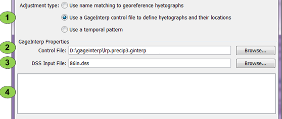
1 | Select this to use a GageInterp file for the definition of the hyetograph records as well as the hyetograph georeferencing. |
2 | This is used to specify the GageInterp control file. The associated Browse… button can be used to bring up a file system browser to locate the file. Note: Only the hyetograph locations, the hyetograph pathnames, and optionally, the DSS file containing them is used from the GageInterp file. |
3 | This overrides the file to use for the DSS input file. If left blank the DSS file specified by the GageInterp control file will be used. |
4 | This area will display any errors or warnings that were encountered when processing the GageInterp control file. |
Item | Description |
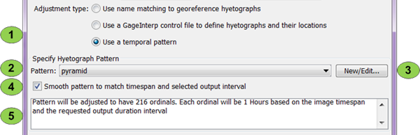
1 | Select this to use a temporal pattern for the disaggregation. |
2 | This dropdown control specifies the pattern to use to disaggregate the TIN. |
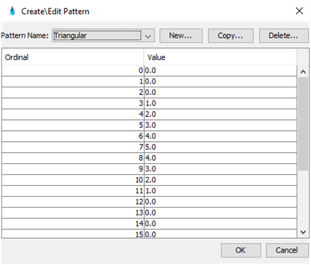
3 | This button is used to access the Pattern Editor, Figure 146, which is used to edit existing patterns and create new ones. Note that any pattern defined is normalized when used so that a pattern with ordinals of [1, 2, 3] will give the same results as a pattern of [100, 200, 300]. |
4 | When this is unchecked, the program will use the pattern ordinal count, along with the timespan defined for the aggregate TIN to determine the timespan of each of the newly created TINs. When the selection is checked, the selected pattern will be resampled to create a valid pattern with the appropriate number of ordinals. |
5 | This area will display information on the resultant pattern and ordinal count that will be used when disaggregating the TIN. |
The Temporal Pattern Editor is similar to the Custom Scale Editor with features such as clicking the right mouse button to insert or delete a value. To help with paste operations, several values can be entered in a single cell and the editor will format them into individual cells automatically.