Total-Load Adaptation Length
There are several options to calculate the total-load adaptation length. The simplest option is to utilize a constant adaptation length calibrate the parameter using field measurements. Experience has shown that for most field applications, this approach is sufficient. However, several other methods are available with varying degrees of complexity. The total-load adaptation length may also be determined.
The advection coefficient considers several processes which affect the velocity and direction of the sediment transport including the vertically non-uniform distribution of the horizontal current velocity and sediment concentration profiles and bed-slope effects.
There are four methods for calculating the total load adaptation coefficient in HEC-RAS:
- Constant adaptation length
2.Weighted average of bed- and suspended-load adaptation lengths
In the case that a constant adaptation length is specified, the total-load adaptation coefficient is computed as
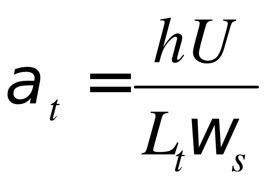 (2 78)
where
 = water depth [L]
 = current velocity [L/T]
 = total-load adaptation length [L]
 = sediment fall velocity [L/T]
The fall velocity is equal to the transport grain size, for single size sediment transport, or the median grain size, in the case of multiple-sized sediment transport.
A more realistic approach to use a transport weighted average of the bed- and suspended-load adaptation lengths (Wu 2007)
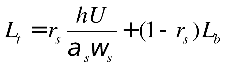 (2 79)
where  is the suspended-load adaptation coefficient,
  is the bed load adaptation length, and
  is the fraction of suspended load of the total load. The methods for determining and are described in subsequent sections.
Bed-load Adaptation Length
There are two options for the bed-load adaptation length. The first is for the user to specify a constant value. There are two methods for calculating the total load adaptation coefficient in HEC-RAS:
- Constant bed-load length
- Depth-dependent method
In the case of the depth-dependent method, the adaptation length is computed as
 (2 80)
where
 = depth-dependent factor approximately between 5 to 10 [-]
 = water depth [L]
Suspended-load Adaptation Coefficient
There are three options for computing the suspended-load adaptation coefficient:
- Constant coefficient
- Zhou and Lin (1998)
- Armanini and Di'Silvio
The figure below shows two examples of the two formulations for the suspended-load adaptation coefficient.
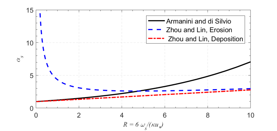
<ac:structured-macro ac:name="anchor" ac:schema-version="1" ac:macro-id="54fcca9d-dc6c-4650-9e60-089bb62fa498"><ac:parameter ac:name="">_Toc53565299</ac:parameter></ac:structured-macro>Figure 2 13. Suspended-load adaptation (adjustment) coefficient.
In the case of the Zhou and Lin (1998) formulation, the adaptation coefficient is computed by solving a 2DV advection-diffusion equation of suspended load with constant diffusivity and uniform flow. A concentration bottom boundary condition is specified for the erosion case, and a gradient boundary condition for the deposition case. The analytical solution is given by
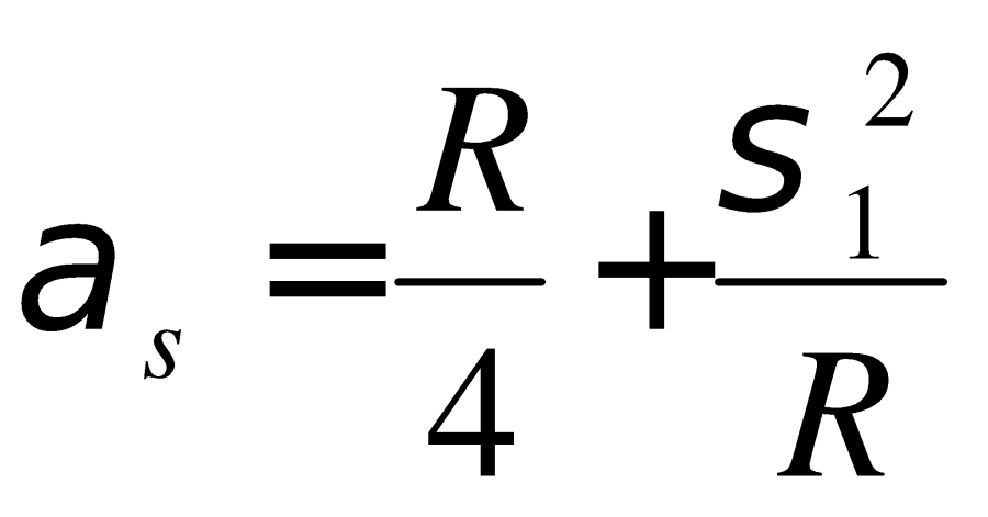 (2 81)
where
 = suspension parameter [-]
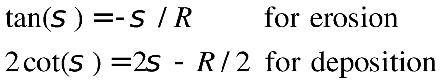
 = first positive root of the following equations:
A plot of the suspended-load adaptation coefficient following Zhou and Lin (1998) is shown in the figure below. The adaptation coefficients for erosion and deposition can be very different, especially for low suspension parameter values. In practice, a weighted average of the erosion and deposition values is used in order to avoid stability issues. It is also noted that the adaptation coefficient of Zhou and Lin (1998) is always greater than 1.
Armanini and Di'Silvio (1986) proposed the following formula for the adaptation coefficient
 (2 82)
where
 = sediment particle settling velocity [L/T]
 = thickness of the bottom layer [L]
 = roughness length [L]
 = total bed shear velocity [L/T]
 = water depth [L]