Bed Sorting and Layering

Bed sorting is the process in which the bed material changes size composition (fraction of each grain size class). The bed is discretized into multiple layers to consider the heterogeneity of bed material size composition along the bed depth (see figure below). The fraction of each grain class is calculated and stored in each layer. The sorting of sediments is calculated with the active or mixing layer concept (Hirano 1971; Karim and Kennedy 1982; Wu 1991; Wu 2004). The active layer is the top layer of the bed which exchanges directly with the sediment moving in the water column. In other words, only the sediment in the mixing layer exchanges with the moving sediment in the water column; whereas, the sediment in the subsurface layers below the active layer does not directly exchange or contact with the moving sediment.

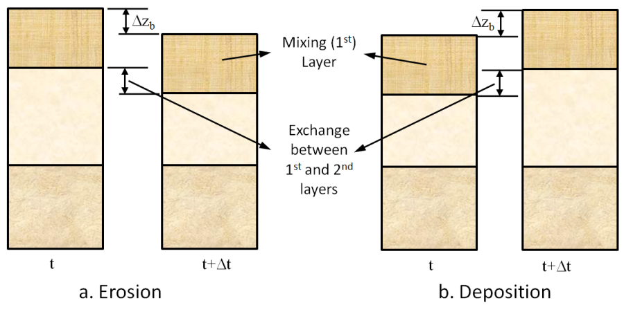
Figure 1. Multiple bed-layer model of bed material sorting (Wu 2007).

There exist several multiple bed layer models in literature (e.g. Spasojevic and Holly 1993; Wu 1991; Lin 2010; Brown 2012; Lai 2020; Wu 2004). Here a new approach is developed based on the work of Wu (1991) and modified for variable bed and grain densities. The bed sorting and layering model solves for fractional sediment mass concentrations in each layer defined as

1)	$\begin{array}{l}\displaystyle m_{jk} = f_{jk}ρ_{dj}\end{array}$

where

$\begin{array}{l}m_{jk}\end{array}$ : fractional mass concentration in layer j and grain class k [M/L³]

$\begin{array}{l}f_{jk}\end{array}$ : grain class fraction by weight in layer j and grain class k [-]

$\begin{array}{l}\rho_{dj}\end{array}$ : dry bulk density of layer j [M/L³]

It is straightforward to see that the sum of the fractional mass concentrations is equal to the dry bulk density

2)	$\begin{array}{l}\displaystyle ρ_{dj} = \sum_{k}m_{jk}\end{array}$

The fractional mass concentrations, m_jk, are analogous to the total-load fractional mass concentrations, C_tk, solved with the transport equation. With the above definitions, the equations describing the bed layer thickness, porosity, and gradation of the first and second layers are given by

3)	$\begin{array}{l}\displaystyle \delta _{1}=\max \left(f_{1,90}d_{90},0.5\Delta \right)\end{array}$

4)	$\begin{array}{l}\displaystyle \frac{\partial \delta _{2}}{\partial t}=\frac{\partial z_{b}}{\partial t}-\frac{\partial \delta _{1}}{\partial t}\end{array}$

5)	$\begin{array}{l}\displaystyle \frac{\partial (m_{1k}\delta _{1})}{\partial t}+m_{*k}\frac{\partial \delta _{2}}{\partial t}=\rho _{sk}(1-\phi _{b})\left(\frac{\partial z_{b}}{\partial t}\right)_{k}\end{array}$

6)	$\begin{array}{l}\displaystyle \frac{\partial (m_{2k}\delta _{2})}{\partial t}=m_{*k}\frac{\partial \delta _{2}}{\partial t}\end{array}$

where

$\begin{array}{l}\delta_1\end{array}$ : first layer thickness [L]

$\begin{array}{l}\delta_2\end{array}$ : second layer thickness [L]

$\begin{array}{l}f_{1,90}\end{array}$ : user-specified active layer scaling factor (typically 1 to 10) [-]

$\begin{array}{l}d_{90}\end{array}$ : 90^th percentile diameter [L]

$\begin{array}{l}\Delta\end{array}$ : bedform height [L]

$\begin{array}{l}z_b\end{array}$ : bed elevation with respect to the vertical datum [L]

$\begin{array}{l}\rho_{sk}\end{array}$ : grain density [M/L³]

$\begin{array}{l}\phi_b\end{array}$ : porosity of the eroded and deposited material [-]

$\begin{array}{l}m_{1k}=f_{1k} \rho_{d1}\end{array}$ : fractional mass concentration in the first (active) layer [M/L³]

$\begin{array}{l}m_{2k}=f_{2k} \rho_{d2}\end{array}$ : fractional mass concentration in the in second layer [M/L³]

$\begin{array}{l}m_{*k}=\begin{cases} m_{1k}\,\,\mathrm{for}\,\,\partial (z_{b} - \delta _{1})/\partial t \geq 0\\ m_{2k}\,\,\mathrm{for}\,\,\partial (z_{b} - \delta _{1}) / \partial t< 0 \end{cases}\end{array}$ [M/L³]

The approach allows for variable bed density and grain density and is also computationally efficient. For the case when the bed porosity and grain density are constant, the above equations reduce to the equations proposed by Wu (2004). It is noted that there is no material exchanged between the sediment layers below the second layer. Solving for the fractional mass concentrations in each bed layer is more convenient than solving for volumes because the total volume of a bed layer is not conserved while the total mass is conserved. In addition, the sum of the fractional mass concentrations directly produces the dry bulk density which is utilized for computations such as consolidation.