The total roughness may be computed from the user-specified Manning's roughness coefficient or computed internally from the individual components. The total bottom roughness may be separated into roughness's due to (1) grains, (2) sediment transport, and (3) bedforms. The bedform roughness may be further divided into roughness's due to: (1) ripples, (2) mega-ripples, and (3) dunes. The grain-related roughness is the skin roughness caused by the sediment grains on the bed. It is necessary for many of the sediment transport formulas. The sediment transport roughness is a friction loss caused by the moving particles near the bed. The transport roughness is usually small compared to the other components. The bedform roughness is the form roughness and can have a large range of values. Bedforms geometry is very difficult to predict and therefore, the bedform roughness has a large uncertainty.

Roughness Specification and Conversion

The total bottom roughness is specified in HEC-RAS with the Manning’s roughness coefficient. It is important to note that the bed roughness is assumed constant in time and not changed according to bed composition and bedforms. This is a common engineering approach which can be justified by the lack of data to initialize the bed composition and the large error in estimating the bed composition evolution and bedforms. In addition, using a constant bottom roughness simplifies the model calibration. The bed roughness used for hydrodynamics may not be the same as that which is used for the sediment transport calculations.  This is because each sediment transport formula was developed and calibrated using specific methods for estimating bed shear stresses or velocities, and these cannot be easily changed. The choice of what roughness parameter is specified and kept constant over an area has important consequences on the flow and its distribution with respect to the water depth (see figure below). The Nikuradse roughness height k_s is related to the roughness length by (Christoffersen and Jonsson 1985)

where

$//<![CDATA[ \begin{array}{l}u_{*}\end{array} //]]>$ = bed shear velocity [L/T]

$//<![CDATA[ \begin{array}{l}k_s\end{array} //]]>$ = Nikuradse roughness [L]

$//<![CDATA[ \begin{array}{l}ν\end{array} //]]>$ = water kinematic viscosity [L²/T]

For flat beds consisting of fine sands or mud, the flow is hydraulically smooth or transitional while beds with coarse sands, gravel, or bedforms are hydraulically rough (Soulsby 1997). Most natural river and coastal flows are hydraulically rough for which case the above equation simplifies to

The equation is based on a logarithmic velocity profile and covers smooth, transitional, and rough turbulent flows.

Assuming rough turbulent flow, the second part of the equation may be ignored, in which case the Colebrook-White equation may be used to convert the roughness height to a Manning’s coefficient as

where

$//<![CDATA[ \begin{array}{l}A=\begin{cases} 1\,\,\,\,\,\,\mathrm{for}\,\mathrm{SI}\,\text{units}\\ 1.486\,\,\mathrm{for}\,\text{English}\,\text{units} \end{cases}\right.\end{array} //]]>$

$//<![CDATA[ \begin{array}{l}R\end{array} //]]>$ = hydraulic radius or water depth [L]

$//<![CDATA[ \begin{array}{l}k_s\end{array} //]]>$ = roughness height [L].

Grain-related Roughness

The grain-related roughness may be estimated as (e.g. Meyer-Peter and Muller 1958)

where

$//<![CDATA[ \begin{array}{l}α_{g,X}\end{array} //]]>$ = Grain-related roughness height coefficient

$//<![CDATA[ \begin{array}{l}d_{X}\end{array} //]]>$ = Diameter corresponding to the X percentile

Examples values of α_g, X from literature are shown in the table below.

Table 25. Grain-related roughness height coefficient.

Reference	dX	αg, X
Ackers and White (1973)		1.23
Meyer-Peter and Muller (1948)		1.0
Engelund and Hansen (1972) Nielsen (1992)		2.50
Strickler (1970)		3.3
Engelund and Hansen (1967), Wilcock (2001) and Wilcock and Crowe (2003)		2.0
Limerinos (1970)		2.8
Kamphius (1974)		2.0
van Rijn (1984c)		3.0

In HEC-RAS, the grain roughness height formulations utilized from the above table are van Rijn (1984c)

The grain-related Manning’s roughness coefficient may be estimated as

where

$//<![CDATA[ \begin{array}{l}d_X\end{array} //]]>$ = Xth percentile diameter [m]

$//<![CDATA[ \begin{array}{l}A_{n,X}\end{array} //]]>$ = Grain-related Mannings n corresponding to d_X [1/(s m^1/6)]

The table below shows some examples of A_n from literature.

Table 26. Grain-related Manning’s coefficient.

Reference
Strickler (1923)		25.6
Li and Liu (1963)		20
Patel and Ranga Raju (1996)		24
Meyer-Peter and Muller (1948)		26

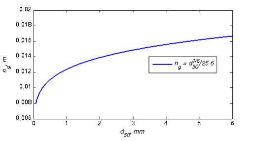
Figure 2 3. Example grain Manning's roughness coefficient following Strickler (1923). 

Limerinos

Limerinos (1956) developed a bed roughness predictor based on data from 11 gravel-bed streams in California as (see Figure below)

where

$//<![CDATA[ \begin{array}{l}A=\begin{cases} 1.219\,\,\,\,\mathrm{for}\,\mathrm{SI}\,\text{units}\\ 1\,\,\,\,\,\,\,\,\,\,\,\,\,\,\mathrm{for}\,\text{English}\,\text{units} \end{cases}\right.\end{array} //]]>$

$//<![CDATA[ \begin{array}{l}n_g\end{array} //]]>$ = grain-related Manning’s roughness coefficient [s/m^1/3]

$//<![CDATA[ \begin{array}{l}R\end{array} //]]>$ = hydraulic radius [L]

$//<![CDATA[ \begin{array}{l}d_{84}\end{array} //]]>$ = 84th percentile diameter [L]

The equation is applicable to high in-bank flows in straight, gravel-bed channels. All the data used corresponded to Froude numbers less than 1. The Limerinos equation only accounts for the grain roughness in gravel-bed streams and does not include other contributions. Therefore, it may be used as the base value in the Cowan (1956) method.

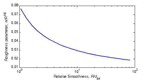
Figure 2 4. Grain roughness using the Limerinos (1956) equation.

It is noted that none of the expression above account for the full distribution of sediments and only consider a representative diameter. This is a limitation of the expressions when being applied to poorly sorted bed material.

Sediment Transport Roughness

Moving sediment produces a roughness due to the energy losses in transporting the sediment. This process is poorly understood and relatively few expressions are available in literature to account for this process. Here two simple formulas are available which account for the added roughness of bed-load transport. The formulas included here for sediment transport roughness are:

1. Wilson (1966)
2. Wiberg and Rubin (1989)

Wilson (1966)

A commonly used formula for the sediment transport related roughness is the Wilson formula (Wilson 1966, 1989ab)

where

$//<![CDATA[ \begin{array}{l}\theta '\end{array} //]]>$ = $//<![CDATA[ \begin{array}{l}\frac{\tau '_{b}}{g(\rho _{s}-\rho )d}\end{array} //]]>$ = grain-related Shields number [-]

$//<![CDATA[ \begin{array}{l}d\end{array} //]]>$ = grain size diameter [L]

The above formula has been used by Camenen and Larson (2007) and others. The above equation must therefore be solved simultaneously with the expressions for the bottom shear stress because the roughness depends on the stress. The exact solution is approximated here using explicit polynomial fits in order to avoid time-consuming iterations in calculating the bed shear stress.

Wiberg and Rubin (1989)

Wiberg and Rubin (1989) proposed the following formula for the sediment transport related roughness

where

$//<![CDATA[ \begin{array}{l}k_{s, s}\end{array} //]]>$ = sediment transport related roughness height [cm]

$//<![CDATA[ \begin{array}{l}d_{50}\end{array} //]]>$ = median grain size [cm]

$//<![CDATA[ \begin{array}{l}τ'_b\end{array} //]]>$ = grain shear stress [M/L/T²]

$//<![CDATA[ \begin{array}{l}τ_{cr}\end{array} //]]>$ = critical shear stress [M/L/T²]

$//<![CDATA[ \begin{array}{l}α_{WS}\end{array} //]]>$ = $//<![CDATA[ \begin{array}{l}0.056\end{array} //]]>$ [ - ]

$//<![CDATA[ \begin{array}{l}a_1\end{array} //]]>$ = $//<![CDATA[ \begin{array}{l}0.68\end{array} //]]>$ [ - ]

$//<![CDATA[ \begin{array}{l}a_2\end{array} //]]>$ = $//<![CDATA[ \begin{array}{l}0.0204\ln(100d_{50})^2 + 0.022\ln(100d_{50}) + 0.0709 (~0.27)\end{array} //]]>$ [ - ]

The formula is based on the hypothesis that the transport roughness is directly proportional to the thickness of the bed-load layer proposed by Owen (1964). The formula is basically that of Dietrich (1982) with recalibrated coefficients.

Bedform Roughness 

Ripple Roughness

The ripple roughness may be estimated as (see Grant and Madsen 1982; Nielson 1992; and Soulsby 1997)

where

$//<![CDATA[ \begin{array}{l}k_{s,r}\end{array} //]]>$ = ripple roughness height [L]

$//<![CDATA[ \begin{array}{l}α_r\end{array} //]]>$ = \text{ripple roughness coefficient on the order of 10 [ - ]}

$//<![CDATA[ \begin{array}{l}\Delta _{r}\end{array} //]]>$ = \text{ripple height }[L]

$//<![CDATA[ \begin{array}{l}λ_r\end{array} //]]>$ = \text{ripple length }[L]

Examples values of α_r from literature presented in the table below.

Table 27. Ripple Roughness Height Coefficient.

Reference
Grant and Madsen (1982)	27.7
Nielsen (1992)	8
Raudkivi (1997)	21.7
Soulsby (1997)	7.5
van Rijn (1993)	10

Dune Roughness

For dunes van Rijn (1984c) method is given by

where

$//<![CDATA[ \begin{array}{l}γ_d\end{array} //]]>$ = dune shape coefficient (~1.0) [ - ]

$//<![CDATA[ \begin{array}{l}\Delta _{d}\end{array} //]]>$ = dune height [L]

$//<![CDATA[ \begin{array}{l}λ_d\end{array} //]]>$ = \text{dune length }[L]

The dune shape coefficient, γ_d, is approximately 1.0 for dunes with angle-of-repose faces as considered in van Rijn (1984c). Dunes with more gently sloping faces have smaller shape coefficients as is common in the field. Van Rijn (1993) proposed setting γ_d = 0.7 based on various field measurements of river systems. van Rijn (1984c) provided expressions for calculating the dune height and length and are shown in Equations (2-94) and (2-95). The figure below shows the dune roughness based on van Rijn (1984c) as a function of the sediment transport stage.

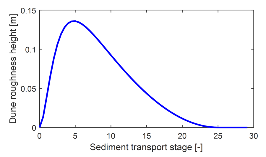
Figure 2 5. Dune roughness height based on van Rijn (1984a).