The area-averaged sediment erosion rate is computed as a function of the erosion potential

E_tk = f_1kE_tk^*

where

E_tk = erosion rate [M/L²/T]

f_1k = active grain class fractions by weight [-]

E_tk^* = potential erosion rate [M/L²/T]

The active layer grain class fractions represent the sediment availability. The erosion potential consists of two components due to (1) hydraulic flow and (2) sheet and splash erosion:

E_tk^* = r_A^SSE_tk^* HF + r_A^SSE_tk^* SS

where

r_A^SS = fraction of horizontal area corresponding to sheet and splash erosion [-]

r_A^HF = fraction of horizontal area corresponding to hydraulic flow erosion [-]

E_tk^SS = sheet and splash erosion rate [M/T/L²]

E_tk^HF = hydraulic flow erosion rate [M/T/L²]

The incorporation of r_A^SS and r_A^HF in the above formulation is important since the present model is designed to support partially hydraulically wet and dry cells. It is noted that r_A^SS + r_A^HF + r_A^NE = 1 where r_A^NE represents the fraction of non-erodible surface area (i.e. bed rock, concrete surface, structures) and surface cover (e.g. vegetation). In the current version of the model, r_A^NE is assumed to be zero.

Hydraulic Flow Erosion

Cohesive Sediments

At low shear stresses, erosion occurs due to particle and small aggregate detachment, while at high shear stresses, erosion occurs primarily due to detachment of clasts or chunks of material and is referred to as “mass erosion” or “mass wasting”. This behavior may be captured by using different erodibility coefficients and critical shear stresses for surface and mass erosion:

$//<![CDATA[ \begin{array}{l}E_{tc}^{*HF}=\begin{cases}0\,\,\,\,\,\,\,\,\,\,\,\,\,\,\,\,\,\,\,\,\,\,\,\,\,\,\,\,\,\,\,\,\,\,\,\,\,\,\,\,\,\,\,\,\,\,\,\,\,\,\,\,\,\,\,\,\,\,\,\,\,\,\,\,\,\,\,\,\,\,\,\,\,\,\mathrm{for}\,\,\tau _{b}\leq \tau _{ce}\\ M\left(\tau _{b}/\tau _{ce}-1\right)\,\,\,\,\,\,\,\,\,\,\,\,\,\,\,\,\,\,\,\,\,\,\,\,\,\,\,\,\,\,\,\,\,\,\,\,\,\,\,\,\,\,\,\,\,\,\,\mathrm{for}\,\,\tau _{ce}< \tau _{b}\leq \tau _{cM}\\ M\left(\tau _{cM}/\tau _{ce}-1\right)+M_{M}\left(\tau _{b}-\tau _{cM}\right)/\tau _{ce}\,\,\,\mathrm{for}\,\,\tau _{b}>\tau _{cM} \end{cases}\right.\end{array} //]]>$

where

E_tc^* HF = cohesive erosion rate [M/L²/T]

τ_b = bed shear stress [M/L/T²]

τ_ce = critical shear stress for cohesive sediment erosion [M/L/T²]

τ_cM = critical shear stress for mass wasting erosion [M/L/T²]

M = surface erosion rate coefficient [M/L²/T]

M_M = erodibility coefficient for mass wasting erosion [M/L²/T]

In other words, different values for the erosion coefficient are specified at different ranges of bed shear stress. If the coefficients M and M_M are equal then the above formulations reduces to the classic linear formulation by Ariathurai (1974) Ariathurai and Arulanandan (1978) based on the data of the data from Partheniades (1962)

$//<![CDATA[ \begin{array}{l}E_{tc}^{*HF}=\begin{cases} 0\,\,\,\,\,\,\,\,\,\,\,\,\,\,\,\,\,\,\,\,\,\,\,\,\,\,\,\,\,\,\mathrm{for}\,\,\tau _{b}\leq \tau _{ce}\\ M\left(\tau _{b}/\tau _{ce}-1\right)\,\,\,\mathrm{for}\,\,\tau _{ce}< \tau _{b} \end{cases}\right.\end{array} //]]>$

where

E_tc^* HF = cohesive erosion rate [M/L²/T]

M = surface erosion rate coefficient [M/L²/T]

Noncohesive Sediments

The hydraulic flow erosion is simulated using the adaptation formulation (see Wu et al. 2007 and references therein).

E_tk^* HF = α_tkω_skC_tk^*

where

α_tk = adaptation coefficient [-]

ω_sk = sediment settling velocity [L/T]

C_tk^* = q_tk^*/(hU) = sediment concentration potential [M/L³]

q_tk^* = total-load sediment transport [M//L/T]

It is noted that if the bed consists of both cohesive and noncohesive sediments, then the erosion potential of noncohesive sediments is limited to that of the noncohesive sediments (see also Brown et al. 2014). This is so that the erosion of noncohesive sediment fractions is never larger than that of the cohesive fractions. One advantage of the adaptation coefficient compared to near-bed sediment concentration potential formulations, is that there are many formulations for the sediment transport potential as compared to the near-bed sediment concentration potential. It also makes it easier to compare model results with Exner type models since for uniform equilibrium conditions they should produce the same transport rates. The main disadvantage of the adaptation approach is that it introduces an additional calibration parameter.

When simulating mixed cohesive and noncohesive sediments, the erosion rates for noncohesive sediments are always computed with the transport formulas for noncohesive sediments but with corrections to the critical shear stress or velocity. In addition, the erosion rates for noncohesives grain classes are limited using the cohesive sediment erosion rate.

Splash and Sheet Flow Erosion

Splash and sheet flow erosion occurs in the “hydraulically dry” portion of the domain which is above the water surface elevation but has precipitation and surface runoff. The region is often referred to simply as the inter-rill region. The splash and sheet flow erosion are computed with a modified form of the rangeland erosion formula developed by Wei et al. (2009)

^{$//<![CDATA[ \begin{array}{l}E_{rk}^{*SS} = r_{E,k}K_{SS}r^{1.052}v^{0.592}\end{array} //]]>$}

where

$//<![CDATA[ \begin{array}{l}K_{SS } = \text{splash and sheet erodibility coefficient (dimensional)}\end{array} //]]>$

$//<![CDATA[ \begin{array}{l}r_{E,k } = \text{grain size function of eroded material (described in a later section) [ - ]}\end{array} //]]>$

$//<![CDATA[ \begin{array}{l}r_{ } = \text{precipitation intensity }[L/T]\end{array} //]]>$

$//<![CDATA[ \begin{array}{l}v = r − f  = \text{excess precipitation rate }[L/T]\end{array} //]]>$

$//<![CDATA[ \begin{array}{l}f_{ } = \text{infiltration rate }[L/T]\end{array} //]]>$

The splash and sheet flow erosion potential formula has been modified for non-uniformly sized sediment by including a grain size function. The function determines the sediment gradation of the eroded material. A simple formulation is proposed as a function of the sediment fall (settling) velocity:

$//<![CDATA[ \begin{array}{l}r_{E,k}=\begin{cases} 0\,\,\,\,\,\,\,\,\,\,\,\,\,\,\,\,\,\,\,\,\,\,\,\,\,\,\,\,\mathrm{for}\,d_{k}>d_{sand}\\ \frac{\omega _{sk}^{-m}}{\frac{1}{N_{sand}}\sum _{i=1}^{N}\omega _{si}^{-m}}\,\,\,\,\mathrm{for}\,d_{k}\leq d_{sand}\,\, \end{cases}\right.\end{array} //]]>$

where

ω_sk = settling velocity for grain class k [L/T]

d_sand = grain size threshold equal to 2 mm [L]

N_sand = number of grain classes smaller than d_sand [-]

m = empirical coefficient between 0 and 0.5 (default = 0.2) [-]

It is assumed that only grains smaller than d_sand= 2 mm are eroded by sheet and splash erosion. If the coefficient m is set to 0, then all of the grain classes with diameters less than d_sand have equal erosion potential. The figure below shows an example of the sheet and splash erosion grain size function.

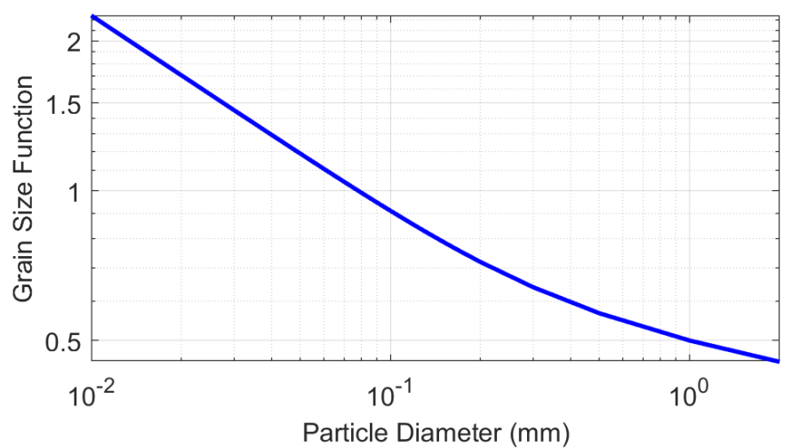
Figure 2 8. Example sheet and splash erosion grain size function with m = 0.2 and the fall velocity computed from Cheng (1997). 

The above approximation is a necessary one for non-uniform sediments because without it the sheet and splash erosion formulations can produce extremely unrealistic erosion gradations for sediment beds with coarse material. Additional research is needed to better extend existing sheet and splash erosion formulas to graded sediments.