Total-load Correction Factor
The total-load correction advection coefficient, βtk, accounts for the vertical distribution of the suspended sediment concentration and velocity profiles, and the generally slower bed-load velocity compared to the depth-averaged current velocity (see figure below) (Wu 2007).
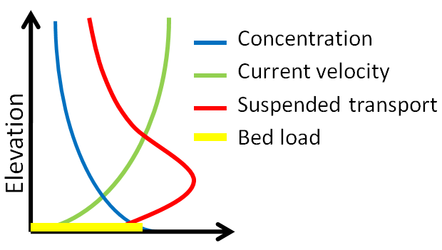
Figure 2.9: Schematic of sediment and current velocity profiles.
The total-load correction factor is given by
| 1) |
\beta _{tk}=\frac{1}{r_{sk}/\beta _{sk}+(1-r_{sk})/\beta _{sk}} |
where
rsk= fraction of suspended-load [-]
βsk= suspended-load correction factor [-]
βbk = bed-load correction factor [-]
It is noted that the sediment transport is assumed to be in the same direction as the flow. Therefore, the influence of the bed-slope on the bedload is not included here. This effect is included separately in the model as an additional term in the bed-change equation. The user is given several options on how to compute the total-load correction factor including specifying a constant or computing it from the bed- and suspended-load correction factors which also may be computed with one of several methods or specified as a constant.
Suspended-load Correction Factor
The suspended-load correction factor is defined as the ration between the vertically integrated suspended-load transport and the transport computed as the simple product of the current velocity times the averaged sediment concentration:
| 2) |
\beta _{sk}=\frac{\int _{0}^{h}uc_{k}dz}{UhC_{k}} |
For fine cohesive sediments, βsk is close to unity while for coarse sediments it is typically between 0.5 and 0.7. There are several options available for computing the suspended-load correction factor. The simplest is a user-specified constant. Two additional options are based on assuming vertical profiles for the current velocity and sediment concentration profiles. By assuming logarithmic current velocity and exponential suspended sediment concentration profiles, an explicit expression for the suspended-load correction factor can be obtained as (Sánchez and Wu 2011b)
| 3) |
\beta _{sk}=\frac{\mathrm{E}_{1}(\phi _{k}A)-\mathrm{E}_{1}(\phi _{k})+\ln (A/Z)\mathrm{e}^{-{\phi _{k}}A}-\ln (1/Z)\mathrm{e}^{-{\phi _{k}}}}{\mathrm{e}^{-{\phi _{k}}A}\left[\ln (1/Z)-1\right]\left[1-\mathrm{e}^{-{\phi _{k}}(1-A)}\right]} |
where
ϕk = ωskh/εvk [-]
A = a/h [-]
Z = z0/h [-]
u = stream-wise current velocity [L/T]
ωsk = sediment settling velocity for size class k L/T]
εvk = vertical mixing (diffusivity) coefficient [L2/T]
a = reference height for the suspended load equal to the thickness of bed-load layer [L]
za = apparent roughness length [L]
\mathrm{E}_{1}(x)=\int _{x}^{\infty }\frac{e^{-t}}{t}dt = exponential integral
The equation can be further simplified by assuming that the reference height is proportional to the roughness height (e.g. a = 30z0 ), so that βsk = βsk(Z,ϕk). Figure 3.4 shows a comparison of the suspended-load correction factor based on the logarithmic velocity with exponential and Rouse suspended sediment concentration profiles.
(a) 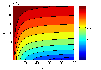 | (b) 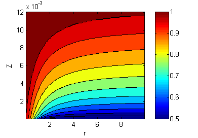 |
|
|
Figure 2 10. Suspended-load correction factors based on the logarithmic velocity profile and (a) exponential and (b) Rouse suspended sediment profiles. The Rouse parameter is r = ωs/(κu*).
Bed-load Correction Factor
The bed-load advection coefficient is defined as the ration between the bed-load velocity and the depth-averaged current velocity:
| 4) |
\beta _{bk}=\frac{u_{bk}}{U} |
where
ubk = bed-load velocity [L/T]
U = depth-averaged current velocity [L/T]
The bed-load correction factor may be specified as a constant or computed with one of several bed-load velocity formulas (presented in the following section).