Grain Properties

Particles are generally classified into discrete grain classes which are assumed to have the same grain properties. In HEC-RAS, the grain properties utilized are the grain size, density, shape, and roundness.

Grain Size

Natural sediments have a distribution of particle sizes, densities, and shapes. For modeling purposes, sediments are grouped into grain classes. Each grain class is characterized by a name, diameter, particle density, and shape factor. The grain classes do not have to have different characteristics may be different only by their name. This allows the modeler to track the movement of sediments within the domain without having to slightly change their characteristics. Sediment particle size may be characterized by a representative diameter. Since natural sediments are naturally irregular in shape, the particle size is characterized by representative diameter. The nominal diameter is the diameter of a sphere that has the same volume of a particle

1)	$\begin{array}{l}\displaystyle d=\left(\frac{6V}{\pi }\right)^{1/3}\end{array}$

where $\begin{array}{l}V\end{array}$ is the volume of the particle. A commonly used particle diameter is the smallest square sieve opening through which a particle will just pass. For natural sediment particles over the range of about 0.2 to 20 mm, the sieve diameter is approximately 0.9 times the nominal diameter on average (U.S. Interagency Committee, 1957; Raudkivi, 1990). Sediment particles are classified into by their diameter. The table below shows the sediment grain size classification scheme utilized by HEC-RAS.

Table 2 1. Sediment grain size aggregate names utilized in HEC-RAS.

Size Range (mm)	Aggregate Name
0.00098 – 0.004	Clay
0.004– 0.008	Very Fine Silt
0.008 – 0.016	Fine Silt
0.016 – 0.032	Medium Silt
0.032 – 0.0625	Coarse Silt
0.0625 – 0.125	Very fine sand
0.125 – 0.25	Fine Sand
0.25 – 0.5	Medium Sand
0.5 – 1	Coarse Sand
1 – 2	Very Coarse Sand
2 – 4	Very Fine Gravel
4 – 8	Fine Gravel
8 – 16	Medium Gravel
16 – 32	Coarse Gravel
32 – 64	Very Coarse Gravel
64 – 128	Small Cobbles
128 – 256	Large Cobbles
256 – 512	Small Boulders
512 – 1024	Medium Boulders
1024 – 2048	Large Boulders

Density

The sediment particle density or grain density, $\begin{array}{l}\rho_s\end{array}$ , is the mass of sediment per unit volume. For quartz particles it is approximately 2,650 kg/m³ and does not vary significantly with temperature or pressure. The specific weight or unit weight of particles, $\begin{array}{l}\gamma_s\end{array}$ , is the density times the gravitational constant

2)	$\begin{array}{l}\displaystyle \gamma_s = g \rho_s\end{array}$

where g is the gravitational constant. The specific gravity, $\begin{array}{l}s\end{array}$ , is the ratio of the grain density and water density

3)	$\begin{array}{l}\displaystyle s=\frac{\rho _{s}}{\rho _{w}}\end{array}$

When the specific gravity is utilized to specify the grain density a reference water density is utilized computed with a temperature of 4ºC. The table below shows typical specific gravity ranges for different common minerals and rocks.

Table 2. Specific gravity ranges for different minerals and rocks.

Material	Specific Gravity
Quartz	2.6 – 2.7
Limestone	2.6 – 2.8
Basalt	2.7 – 2.9
Magnetite	3.2 – 3.5
Coal	1.3 – 1.5

However, often when the specific gravity is utilized in sediment transport equations it is more appropriate to utilize the ratio of the grain density and the actual water density.

Shape Factor

The particle shape factor utilized is attributed to Corey (1949)

4)	$\begin{array}{l}\displaystyle S_{F}=\frac{c}{\sqrt{ab}}\end{array}$

where

$\begin{array}{l}a\end{array}$ = length of the particle along the long axis perpendicular to the other two axes [L]

$\begin{array}{l}b\end{array}$ = length along the intermediate axis perpendicular to the other two axes [L]

$\begin{array}{l}c\end{array}$ = length along the short axis perpendicular to the other two axes [L]

The shape factor is utilized for some of the sediment fall velocity formulas. The shape factor of natural particles is usually about 0.6 to 0.7.

Roundness

The particle roundness can only be estimated based on the comparison with the images proposed by Powers (1953), shown in the figure below, and the use of Folk's (1955) corresponding scale shown in the table below.

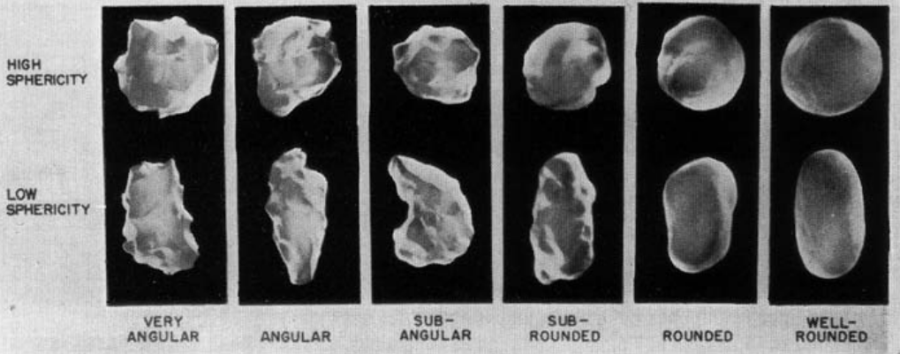
Figure 1. Particle roundness scale proposed by Powers (1953) (from Powers (1953).

Table 3. Folk's (1955) Roundness "rho" Scale.

Powers Verbal Class	Rho Scale Class Intervals
Very angular	0.0 – 1.0
Angular	1.0 – 2.0
Sub-angular	2.0 – 3.0
Sub-rounded	3.0 – 4.0
Rounded	4.0 – 5.0
Well-rounded	5.0 – 6.0

Bulk Properties

Grain-Size Distribution

In general, natural sediments consists of a mixture of sediment sizes, shapes, densities, etc. In the multiple-grain class approach, the sediment mixture is discretized in a fixed number of sediment grain classes, each with own grain properties. The grain properties are generally different from grain classes to grain class, but they may in fact be the same (i.e. same grain size). In fact, allowing grain classes to have the same properties allows tracking (mapping) of sediments without having to artificially change the grain characteristics, namely grain size. Each grain class, numbered k is defined by an upper and lower bound diameters and a representative grain class diameter represented as $\begin{array}{l}d_{k+1/2}\end{array}$ and $\begin{array}{l}d_{k-1/2}\end{array}$ , respectively. The grain class diameter is defined here as the geometric mean of the bound diameters $\begin{array}{l}d_{k}=\sqrt{d_{k+1/2}d_{k-1/2}}\end{array}$ . Either the representative diameters or bounding diameters may be specified as model input. The grain class limits are only used to compute the sediment percentile diameters (i.e. the sediment percentile diameters are the diameters corresponding to certain percentile such as the 50^th percentile). The algorithm used to compute

The grain class fractions, or percentages are usually measured by weight using a sieving analysis but can be also in units of volume or particle count. The grain class fractions by weight are represented by f_k and fractions by volume by f̂_k. If the grain class particle densities, ρ_sk, are known the fractions can be converted from by volume to by weight as

5)	$\begin{array}{l}\displaystyle \hat{f}_{k}=\frac{\rho _{sk}^{-1}f_{k}}{\sum _{i}\rho _{si}^{-1}f_{i}}\end{array}$

6)	$\begin{array}{l}\displaystyle f_{k}=\frac{\rho _{sk}\hat{f}_{k}}{\sum _{i}\rho _{si}\hat{f}_{i}}\end{array}$

Most of the grain fractions utilizes in this report represent weight fractions and both the input and output grain fractions are fractions by weight.

The grain-size distribution of a sediment mixture can be represented by a histogram of grain class fractions and a cumulative frequency curve (Krumbein 1934). An example of a grain-size distribution is shown in the figure below.

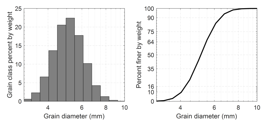
Figure 2. Grain-size distribution histogram (left) and cumulative frequency curve (right).

Many natural sediments have a grain-size distribution which can be approximated by a log-normal distribution. The example grain-size distribution above follows a log-normal distribution. When plotted on a log-scale, the log-normal distribution has an approximate normal (Gaussian) distribution curve.

Characteristic Diameters

The grain size distribution commonly described with by percentile diameters. These diameters correspond to a specific percent by weight finer on the cumulative frequency curve. For example, the 50^th percentile (median) diameter, d₅₀, is the particle diameter at which 50% by weight of the same is finer. More generally, the notation d_n represents the diameter at which n percent by weight is finer. Other commonly used percentile diameters are d₁₀, d₁₆, d₃₅, d₅₀, d₆₅, d₈₄, and d₉₀. When interpolating the percentile diameters from the cumulative frequency curve it is usually done in log-space for the grain diameters. Other commonly used representative grain diameters are the arithmetic mean diameter, d_m, and the geometric mean diameter, d_g, defined respectively as

7)	$\begin{array}{l}\displaystyle d_m = \Sigma_k f_k d_k\end{array}$

8)	$\begin{array}{l}\displaystyle d_g = exp(\Sigma_k f_k \ln(d_k))\end{array}$

Uniformity

The uniformity of a sediment grain size distribution is a measure of how well sorted the distribution is. The uniformity or sorting is often described can be described by the geometric standard deviation

9)	$\begin{array}{l}\displaystyle \sigma _{g}=\exp \sqrt{\sum _{k}f_{k}(\ln d_{k}-\ln d_{g})^{2}}\end{array}$

where

$\begin{array}{l}f_k\end{array}$ = grain class fraction by weight [-]

$\begin{array}{l}d_k\end{array}$ = grain class characteristic diameter [L]

$\begin{array}{l}d_g\end{array}$ = geometric mean [L]

The following table describes the sorting classifications based on the geometric standard deviation

Table 4. Grain-related roughness height coefficient.

Geometric Standard Deviation ( $\begin{array}{l}\sigma_g\end{array}$ )	Classification
Very well sorted	<1.27
Well sorted	1.27 – 1.41
Moderately well sorted	1.41 – 1.62
Moderately sorted	1.62 – 2.00
Poorly sorted	2.00 – 4.00
Very poorly sorted	4.00 – 16.00
Extremely poorly sorted	> 16.00

Porosity

The porosity is a measure of how the volume of voids per unit volume of the deposit

10)	$\begin{array}{l}\displaystyle \phi =\frac{V_{v}}{V}\end{array}$

where

$\begin{array}{l}V_v\end{array}$ = volume of the voids [L³]

$\begin{array}{l}V\end{array}$ = total volume of mixture [L³]

The porosity of sediments depends on the grain size, shape, roundness, sorting, and the level of compactness. The sediment porosity can vary from 0.82 for freshly deposited clays to 0.25 for extremely poorly sorted sediments.

Dry Bulk Density

The two most commonly used bulk densities are the wet and dry bulk densities. The dry bulk density or simply dry density is defined as

11)	$\begin{array}{l}\displaystyle \rho _{d}=\frac{m_{s}}{V}\end{array}$

where

$\begin{array}{l}m_s\end{array}$ = sediment mass [M]

$\begin{array}{l}V\end{array}$ = volume water-sediment mixture [L³]

The dry bulk density can be viewed as a sediment mass concentration. It is a function of the particle densities and the porosity/volume concentration. Dry densities generally vary between

300 to 1,600 kg/m³. The dry bulk density can be calculated for a grain size distribution with a porosity as

12)	$\begin{array}{l}\displaystyle \rho_d = (1 - \phi)\Sigma_k \rho_{sk}\hat{f}_k =(1-\phi)(\Sigma_i \rho_{si}^{-1}f_i)^{-1}\end{array}$

where

$\begin{array}{l}\hat{f}_k\end{array}$ = grain class fraction by volume [-]

$\begin{array}{l}f_k\end{array}$ = grain class fraction by weight [-]

$\begin{array}{l}ρ_{sk}\end{array}$ = grain density [M/L³]

$\begin{array}{l}\phi\end{array}$ = porosity [-]

Download PDF

Sediment Properties

Grain Properties

Grain Size

Density

Shape Factor

Roundness

Bulk Properties

Grain-Size Distribution

Uniformity

Porosity

Dry Bulk Density