The computation of the subgrid bed change, sorting, and layering is done on the sediment subgrid but using the wetted area computed from the hydraulics subgrid. It is possible to develop an algorithm in which the sediment subgrid regions are dynamically adjusted to match the wet/dry interface in a way similar to how the vertical bed layers are treated. However, this approach would require mass transfer (mixing) between adjacent areas as well as merging and splitting of areas. This added complexity and computational costs is not considered worth the benefits and a simpler, faster, albeit slightly less accurate is proposed here. The process of computing the subgrid bed change is illustrated in the schematic below.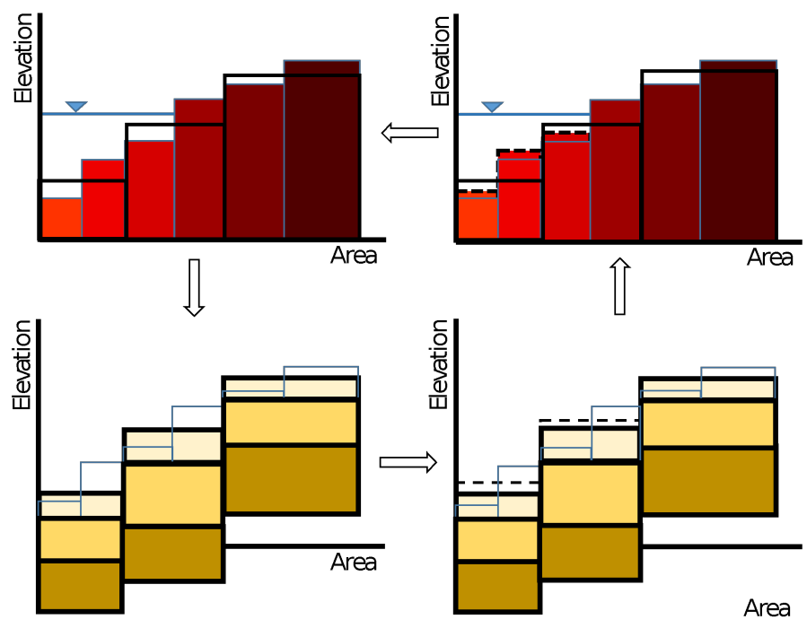

Figure 3 26. Schematic representing computation of bed change.

Subcell Bed Change

The total bed change is computed

1)	$\begin{array}{l}\displaystyle \Delta z_{bi}=\frac{1}{1-\phi _{bi}}\sum _{k}\frac{\Delta M_{bki}}{\rho _{sk}}\end{array}$

where

$\begin{array}{l}\Delta z_{bi}\end{array}$ : bed change for sediment subarea i [L]

$\begin{array}{l}\Delta M_{bki}\end{array}$ : fractional mass exchange with the bed in subarea i [M/L²]

$\begin{array}{l}\phi_{bi}\end{array}$ : porosity of the eroded and deposited material [M/L³]

$\begin{array}{l}ρ_{sk}\end{array}$ : grain class particle density [M/L³]

The fraction a mass exchange is computed as the sum of the mass rates times the scaled time step as

2)	$\begin{array}{l}\displaystyle \Delta M_{bki} = f_{M}\Delta t\left(D_{tki}-E_{tki}+S_{bki}\right)\end{array}$

where

$\begin{array}{l}\Delta M_{bki}\end{array}$ : fractional mass exchange with the bed in subarea i [M/L²]

$\begin{array}{l}D_{tki}\end{array}$ : fractional deposition rate for sediment subarea i [M/L²/T]

$\begin{array}{l}E_{tki}\end{array}$ : fractional erosion rate for sediment subarea i [M/L²/T]

$\begin{array}{l}S_{bki}\end{array}$ : fractional bed-slope term for sediment subarea i [M/L²/T]

$\begin{array}{l}f_{M}\end{array}$ : morphologic acceleration factor [-]

$\begin{array}{l}\Delta t\end{array}$ : time step [T]

Subcell Erosion Potential

The subcell erosion may be computed with one of five methods. The table below summarizes how each method treats the bed and hydrodynamic variables and if the erosion is scaled with the local depth.

Table 3 1. Summary of subcell erosion potential approaches.

Method	Depth-Weighting	Bed Properties	Hydraulics
Constant	None	Cell Wet-Average	Cell Wet-Average
Variable Bed	None	Subcell	Cell Wet-Average
Full Subgrid	None	Subcell	Subcell

In all of the methods the actual local erosion erosion rates are computed using the local grain fractions as

3)	$\begin{array}{l}\displaystyle E_{tki} = f_{1ki}E_{tki}^*\end{array}$

Constant

This is the simplest and most computationally efficient approach. Constant erosion rate potentials are computed for the hydraulically wet and dry portions of a cell using representative (i.e. area-average) bed fractions and properties, hydraulic variables, etc. The local subarea erosion rate potential are then computed as a weighted average of those two rates depending on how much of the sediment subarea is wet. This may be expressed as

4)	$\begin{array}{l}\displaystyle E_{tki}^* = ϕ_i^W E_{tk}^{HF}(f_{1k}^W) + \phi_i^D E_{tk}^{SS}(f_{1k}^D)\end{array}$

where

$\begin{array}{l}E_{tk}^*\end{array}$ : cell fractional erosion rate potential [M/L²/T]

$\begin{array}{l}ϕ_{i}^{W}\end{array}$ : fraction of subarea which is hydraulically wet area [-]

$\begin{array}{l}ϕ_{i}^{D}\end{array}$ : fraction of subarea which is hydraulically dry area $\begin{array}{l}\left( ϕ_{i}^{W} + ϕ_{i}^{D} = 1\right)\end{array}$ [-]

$\begin{array}{l}f_{1k}^{W}\end{array}$ : cell wet area average grain fractions by weight [-]

$\begin{array}{l}f_{1k}^{D}\end{array}$ : cell dry area average grain fractions by weight [-]

The advantage of the above approach is that the erosion potentials only need to be estimated once per cell and not for each cell subarea. However, the approach does not take into account the bed gradation of each subregion.

Variable Bed

In this method, the subarea erosion rates are computed using the local bed gradations and wet-averaged hydrodynamics as

5)	$\begin{array}{l}\displaystyle E_{tki}^* = ϕ_i^W E_{tki}^{* HF}(f_{1ki})+ \phi_i^D E_{tki}^{*SS}(f_{1ki})\end{array}$

where

$\begin{array}{l}E_{tki}^*\end{array}$ : subcell fractional potential erosion rate [M/L²/T]

$\begin{array}{l}E_{tki }^{*HF}(f_{1ki})\end{array}$ : subcell fractional potential erosion rate corresponding to hydraulic flow erosion [M/L²/T]

$\begin{array}{l}E_{tki }^{*SS}(f_{1ki})\end{array}$ : subcell fractional potential erosion rate corresponding to sheet and splash erosion [M/L²/T]

$\begin{array}{l}f_{1ki}\end{array}$ : subcell active layer grain class fractions [-]

$\begin{array}{l}ϕ_{i}^W\end{array}$ : fraction of subarea which is hydraulically wet [-]

$\begin{array}{l}ϕ_{i}^D\end{array}$ = fraction of subarea which is hydraulically dry $\begin{array}{l}\left( ϕ_{i}^W + ϕ_{i}^D = 1 \right)\end{array}$ [-]

In this approach, the sediment erosion potentials are computed for each subarea using cell-averaged hydrodynamic variables along witht the bed gradation for each subarea. Therefore it is significantly more computationaly expensive than assuming constant subcell erosion potentials. However, the erosion potentials are more realistic because they take into account the bed gradation of each subregion.

Full Subgrid

The full subgrid approach computes subcell erosion rates using subcell bed gradations and hydrodynamics:

6)	$\begin{array}{l}\displaystyle E_{tki}^* = {E_{tki}}^({f_{1ki}}^, h_i, u_{*i}, U_i, ~\hdots ~)\end{array}$

where

$\begin{array}{l}E_{tki}\end{array}$ : subcell fractional erosion rate [M/L²/T]

$\begin{array}{l}f_{1ki}\end{array}$ : subcell area active layer grain class fractions [-]

$\begin{array}{l}E_{tki}^*\end{array}$ : subcell fractional potential erosion rate [M/L²/T]

$\begin{array}{l}h_{i}\end{array}$ : subcell water depth [L]

$\begin{array}{l}u_{*i}\end{array}$ : subcell total shear velocity [L/T]

$\begin{array}{l}U_{i}\end{array}$ : subcell current velocity [L/T]

This approach is the most computationally expensive of all the methods because it requires reconstructing the subcell hydrodynamic variables and utilizing the subcell bed composition to compute subcell erosion potentials. However, the erosion potentials are more realistic because they take into account the bed gradation of each subregion.

Subcell Deposition

Sediment deposition is a function of the sediment fall velocity and the sediment concentration. In order to efficiently solve the transport equation implicitly, the sediment deposition is formulated as

7)	$\begin{array}{l}\varpi _{tk}=\begin{cases} \alpha _{tk}\omega _{sk}\,\,\,\mathrm{for}\,\,\text{noncohesives}\\ P_{D}\omega _{sf}\,\,\,\mathrm{for}\,\,\text{cohesives} \end{cases}\right.\end{array}$

where

$\begin{array}{l}\overline{\omega}_{tk}\end{array}$ : fractional deposition rate coefficient [L/T]

$\begin{array}{l}α_{tk}\end{array}$ : total-load adaptation coefficient [-]

$\begin{array}{l}ω_{sk}\end{array}$ : sediment particle settling velocity [L/T]

$\begin{array}{l}P_{D}\end{array}$ : probability of deposition for cohesive sediments [-]

$\begin{array}{l}ω_{sf}\end{array}$ : sediment floc settling velocity [L/T]

There are two approaches for calculating the cell subgrid deposition rate.

Table 32. Summary of deposition approaches.

Method	Depth-Weighting	Capacity-Weighting
Veneer (Constant)	None	None
Depth-Weighted	Yes	None
Capacity-Weighted	None	Yes

Veneer Method

The simplest approach for computing the subgrid deposition rate is to simply assume that the deposition rate is constant within the wet portion of a cell:

8)	$\begin{array}{l}\displaystyle D_{tki} = \phi_i^W ϖ_{th} C_{th}\end{array}$

where

$\begin{array}{l}D_{tki}\end{array}$ : fractional deposition coefficient for sediment subarea i [L/T]

$\begin{array}{l}D_{tk}^{HF}\end{array}$ : fractional deposition rate for sediment subarea i [M/L²/T]

$\begin{array}{l}ϕ_{i}^W\end{array}$ = wet fraction of subarea i (between 0 and 1) [-]

Since it is assumed deposition only occurs in wet portion of cells, the above equation only has one term on the right-hand-side representing the “wet” deposition. The veneer method is the default method because of its simplicity. The method basically assumes that the subgrid sediment concentration is the same as the cell-averaged concentration.

Depth-Weighted Method

Chang (1998) proposed a method for computing the lateral bed change in 1D cross-sections which distributes the total area change as a function of the local excess shear stress. A simpler version of the formula is applied here to the deposition rate by setting the critical shear to zero and assuming a constant friction slope within the cell. This leads to the depth-dependent formulation

9)	$\begin{array}{l}D_{tki}=\begin{cases} \frac{h_{i}^{m} A^W }{\sum_{j}h_{i}^{m}a_{j}^{W}} \varpi _{tk}C_{tk} \,\,\mathrm{for}\,\,h_{i}>0\\ 0\,\,\,\,\,\,\,\,\,\,\,\,\,\,\,\,\,\,\,\,\,\,\,\,\,\,\,\,\,\,\,\,\,\,\mathrm{for}\,\,h_{i}=0 \end{cases}\right.\end{array}$

where

$\begin{array}{l}ϕ_{i}^{W}\end{array}$ : wet fraction of subarea i (between 0 and 1) [-]

$\begin{array}{l}h_{i}\end{array}$ : subarea water depth [L]

$\begin{array}{l}m\end{array}$ : empirical coefficient generally between 0 and 1 (set to 0.6 here) [-]

$\begin{array}{l}a_{i}^{W} = ϕ_{i}^W a_i\end{array}$ : wet area of subarea i [L²]

$\begin{array}{l}a_{i}\end{array}$ : area of subregion i [L²]

$\begin{array}{l}ϕ_{i}^{W}\end{array}$ : fraction of subregion which is wet [-]

$\begin{array}{l}C_{tk}\end{array}$ : cell-average total-load concentration [M/L³]

The above option is similar to the “Reservoir Option” in the HEC-RAS 1D sediment transport model.

Capacity-Weighted Method

Volp (2017) proposed a subgrid deposition method which utilizes the concentration capacity (i.e. equilibrium concentration) to compute subgrid sediment deposition rates. The method assumes that the subgrid sediment concentration tend toward equilibrium. A similar formulation is utilized here as

10)	$\begin{array}{l}D_{tki}=\begin{cases} \frac{C_{tki} A^W}{\sum _{j}C_{tkj}a_{j}^{W}} \varpi _{tk} C_{tk} \,\,\,\mathrm{for}\,\,h_{i}>0\\ 0\,\,\,\,\,\,\,\,\,\,\,\,\,\,\,\,\,\,\,\,\,\,\,\,\,\,\,\,\,\,\,\,\,\,\,\,\,\mathrm{for}\,\,h_{i}=0 \end{cases}\right.\end{array}$

where

$\begin{array}{l}C_{tki*} = f_{1ki} C_{tki}^*\end{array}$ : subgrid equilibrium sediment concentration [M/L³]

$\begin{array}{l}f_{1ki}\end{array}$ : grain class fraction in active layer [-]

$\begin{array}{l}a_{i}^{W} = ϕ_{i}^W a_i\end{array}$ : wet area of subarea i [L²]

$\begin{array}{l}a_{i}\end{array}$ = area of subarea i [L²]

$\begin{array}{l}ϕ_{i}^W\end{array}$ = fraction of subarea which is wet [-]

$\begin{array}{l}C_{tk}\end{array}$ = cell-average total-load concentration [M/L³]

Subcell Wet and Dry Bed Change

Using the total wetted area from the hydraulics area-elevation curve ($\Updelta A^{W}$), the fraction of wetted area on each sediment subarea is calculated as

11)	$\begin{array}{l}\phi _{i}^{W}=\begin{cases}\min \left(\frac{A^{W}}{a_{i}},1\right)\,\,\,\,\,\,\mathrm{for}\,\,i=1\\ \min \left[\frac{1}{a_{i}}\left(A^{W}-\sum _{j}^{i-1}a_{j}\right),1\right]\,\,\,\,\,\,\mathrm{for}\,\,i>1 \end{cases}\right.\end{array}$

where

$\begin{array}{l}ϕ_{i}^W =1 - \phi_i^D\end{array}$ : wetted fraction of subarea i (between 0 and 1) [-]

$\begin{array}{l}ϕ_{i}^D\end{array}$ : dry fraction of subarea of subarea i (between 0 and 1) [-]

$\begin{array}{l}A^W\end{array}$ : total wetted area determined from high-resolution elevation-area curve [L²]

$\begin{array}{l}a_{i}\end{array}$ : area corresponding to subarea i [L²]

It is noted that it is assumed to be no deposition in the dry areas. Once the above fractional erosion and deposition rates are calculated for each subarea, the one-dimensional (1DV) bed-sorting and layering model may be applied. The result from the 1DV model is the fractional and total bed change $\begin{array}{l}\Delta z_{bi}\end{array}$ , dry bulk density ρ_dji, and gradation f_jki for each subarea.

The bed change corresponding to the wet and dry portions of a subarea are determined as

12)	$\begin{array}{l}\displaystyle \Delta z_{bi}^W = \frac{f_{M}\Delta t}{1-\phi _{bi}}\sum _{k}\rho _{sk}^{-1} \left( D_{tki}^{HF} - E_{tki}^{HF} + S_{bki} \right)\end{array}$

13)	$\begin{array}{l}\displaystyle \Delta z_{bi}^{D}=-\frac{f_{M}\Delta t}{1-\phi _{bi}}\sum _{k}\rho _{sk}^{-1}E_{tki}^{SS}\end{array}$

in which

$\begin{array}{l}\Delta t\end{array}$ : time step [T]

$\begin{array}{l}f_{M}\end{array}$ : morphologic acceleration factor [-]

$\begin{array}{l}D_{tk}^{HF}\end{array}$ : hydraulic flow total-load deposition rate [M/T/L²]

$\begin{array}{l}E_{tk}^{HF}\end{array}$ : hydraulic flow total-load erosion rate [M/T/L²]

$\begin{array}{l}E_{tk}^{SS}\end{array}$ : sheet and splash total-load erosion rate [M/T/L²]

$\begin{array}{l}ρ_{dbi}\end{array}$ : dry bulk density of exchange material [M/L³]

The subarea-averaged bed change is therefore

14)	$\begin{array}{l}\displaystyle \Delta z_{bi} = \phi_i^W \Delta z_{bi}^W + \phi_i^D \Delta z_{bi}^D\end{array}$

The next step is to apply the bed change to the high-resolution hydraulics curve. The bed change could directly be applied without consideration of the wet/dry status of the hydraulics curve, but this would lead to artificial artifacts where the dry land is eroded by concentrated flow and vice versa. A simple approach is devised here which avoids this problem.

By applying a simple mass conservation between the two subgrid curves, the bed elevations on the hydraulics elevation-area χ is then updated as

15)	$\begin{array}{l}\displaystyle \Delta z_{b\chi }=\phi _{\chi }^{W}\Delta z_{bi}^W + \phi_{\chi}^D \Delta z_{bi}^D \,\,\,\mathrm{for}\,\,\chi \in i\end{array}$

where

$\begin{array}{l}χ\end{array}$ = subscript indicating hydraulic elevation-area

$\begin{array}{l}i\end{array}$ = subscript indicating sediment subregion
$\begin{array}{l}\phi _{\chi }^{W}=\begin{cases}1\,\,\,\,\,\mathrm{for}\,\,\eta >z_{b\chi }\\ 0\,\,\,\,\,\text{otherwise} \end{cases}\right.\end{array}$
$\begin{array}{l}{A_{}}^{W}\end{array}$ = wetted area determined from high-resolution elevation-area curve [L²]

$\begin{array}{l}a_{i}\end{array}$ = area corresponding to subarea i [L²]

The approach avoids “bleeding” of the bed change across the wet/dry interface.

Download PDF

Subcell Bed Elevations and Bed Change

Subcell Bed Change

Subcell Erosion Potential

Constant

Variable Bed

Full Subgrid

Subcell Deposition

Veneer Method

Depth-Weighted Method

Capacity-Weighted Method

Subcell Wet and Dry Bed Change