There are several sediment transport options which are only available in 2D. The goal is for both 1D and 2D sediment transport to have the same options but for now the 2D only options have been places in a single editor called 2D Options which is available from the Sediment Data editor under the Options menu (see figure below).

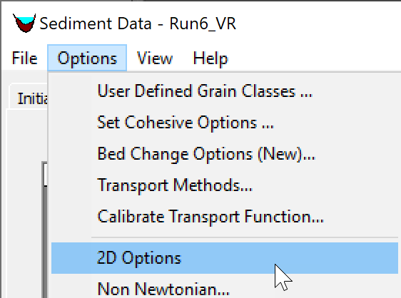
Figure 1. Opening the 2D Options editor from the Sediment Data editor.

The 2D Sediment Options editor is shown in the figure below. The editor is used to specify the options for sheet and splash erosion, the morphologic acceleration factor, the base bed-slope coefficient, and hindered settling.

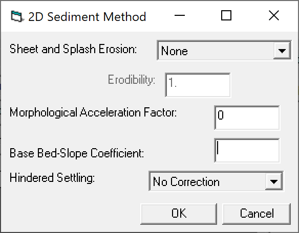
Figure 2. 2D Options editor.

Sheet and Splash Erosion

The first option available in the editor is the Sheet and Splash Erosion. The 2D sediment transport model has the option to use the Wei et al. (2009). The formulation has an erodibility coefficient which for simplicity is set to a single value in HEC-RAS. The units of the erodibility coefficient are kg∙m^-3.644∙s^0.644. Wei et al. (2009) reported values for the sheet and splash erosion coefficient between 1124 and 2555 kg∙m^-3.644∙s^0.644 for 3 grassland rangeland plots in Arizona (all variables in the International System of Units). However, its value can vary by orders of magnitude for different soil types and cover characteristics.

Morphologic Acceleration Factor

The Morphologic Acceleration Factor is a parameter which can be used to turn off the bed change or as the name implies, to accelerate the bed change. The factor is directly multiplied by the mass bed exchange rates at every time step. A value of zero will turn off the bed elevation and bed composition change.
The Morphologic Acceleration Factor can be utilized in several ways. The first and most obvious is to simply turn off updating the bed elevation and bed composition by setting it to a value of zero. This saves computational time and is useful for idealized situations are when debugging a problem with a sediment model.
Another way the factor can be used is as a scaling factor to the morphological change. In other words, the factor can be used to simulate a time period which represents the morphological change of a time period equal to the simulation period times the Morphologic Acceleration Factor. This approach is commonly used in coastal applications with tidal boundary conditions. As an example, a 5-year simulation can be run with Morphologic Acceleration Factor of 20 to simulate 100 years of change which greatly reduces the computational time. However, it should be noted that this approach changes the order of events (i.e. storms and tidal forcing with respect to morphological features) which can have a negative impact on the accuracy of the approach.
Lastly, the Morphologic Acceleration Factor can also be used as a time speed-up factor. This approach is more appropriate in river applications or when simulating single events or sequences of events. As an example, a 20-day simulation can be reduced to 2 days by setting the Morphologic Acceleration Factor to 10 and importantly also speeding up the boundary conditions by the same factor. However, just as in the previous example, care must be taken as to not speed-up the time so much that the hydrodynamics change substantially and thereby the morphological change.
The Morphologic Acceleration Factor should be used with caution as it can lead to misleading results or instabilities. The best practice for using the factor is to test the validity of the factor by doing a full or partial length of a simulation with the factor and without it and compare the results. If the results agree reasonably well, then longer or alterative simulations can usually be done with the Morphologic Acceleration Factor thus saving time. It is generally not recommended to use a factor larger than 30 to 50, and values between but not equal to 0 and 1. The Morphologic Acceleration Factor can be verified by reducing its value (e.g. by a factor of 2) while also increasing the simulation time by the same factor and verifying the simulation results do not significantly change.
Since, the Morphologic Acceleration Factor is applied to the bed exchange rates, the approach does not change total-load transport rates or concentrations. In addition, the approach is not locally mass conservative but approximately globally conservative.
Finally, it is important to emphasis that the Morphologic Acceleration Factor should NOT be used as a calibration parameter. It should be used carefully and validated to make sure the results are not sensitive to the Morphologic Acceleration Factor. When used carefully the Morphologic Acceleration Factor can be a powerful and useful tool in numerical studies.

Base Bed-Slope Coefficient

The Base Bed-Slope Coefficient specifies the maximum value of the bed-slope coefficient. The coefficient is then reduced based on the skin and critical shear stresses. As the ratio between the skin and critical shear stress increases bed-load particles are less influenced by the bed slope. The coefficient is used to compute an additional sediment flux in the downslope direction which is a function of the bed slope, the bedload, and the bed-slope coefficient. For further details on the formulation, the user is referred to the HEC-RAS 2D Sediment Technical Reference manual (HEC 2020). The Base Bed-Slope Coefficient typically has a value between 0.1 and 1. Increasing the coefficient has the effect of smoothing the bathymetry. Measured bed change can be used to calibrate the base bed-slope coefficient. However, its effect is significantly less than the transport formula, transport scaling factors and mobility scaling factor. The Base Bed-Slope Coefficient will tend to improve model stability by smoothing out small scale instabilities. However, if the value is too large the numerical scheme can become unstable. In these situations the user can either reduce the computational time step or reduce the value of the Base Bed-Slope Coefficient.

Hindered Settling

Hindered settling is the condition in which the settling velocity of particles or flocs is reduced due to a high concentration of particles. Hindered settling is primarily produced by particle collisions and the upward water flow equal to the downward sediment volume flux. Hindered settling occurs to both cohesive and noncohesive particles. However, the hindered settling correction described here only applies to noncohesive particles. The hindered settling of cohesive particles is accounted for in the floc settling method. Currently, the 2D sediment has the option to use the Richardson and Zaki (1954) formula for hindered settling (see figure below). For simplicity the exponent in the Richardson and Zaki (1954) is set to 4.0 and cannot be modified in the user interface.

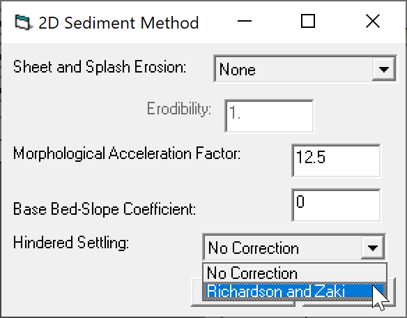
Figure 3. Setting the hindered settling method to the Richardson and Zaki (1954) method.

The figure below shows the ratio of the hindered settling velocity $//<![CDATA[ \begin{array}{l}\omega_{sd}\end{array} //]]>$ and free settling velocity $//<![CDATA[ \begin{array}{l}\omega_{sd0}\end{array} //]]>$ as a function of the total sediment concentration by volume following Richardson and Zaki (1954).

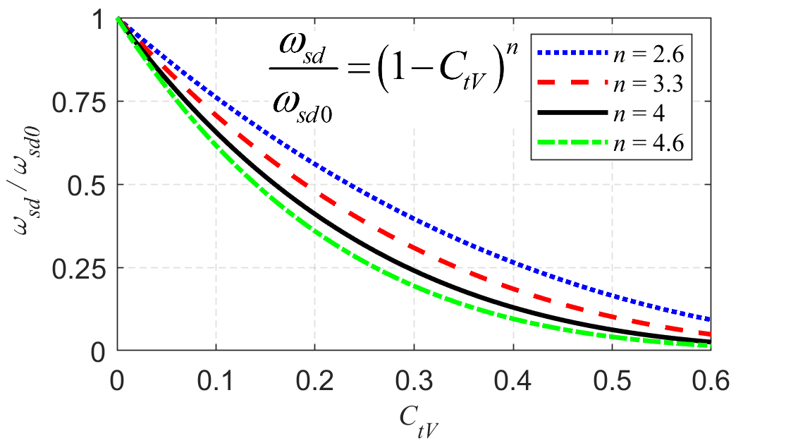
Figure 4. Richardson and Zaki (1954) hindered settling velocity formula.