The second tab on the Sediment Data editor defines sediment boundary conditions (see figure below). The editor automatically lists external model boundaries. HEC-RAS requires a boundary condition at all external boundaries. If any external boundary (i.e. boundary condition line) is left unspecified, then an equilibrium sediment load boundary condition is assumed. The types of boundary conditions which may be specified in a 2D sediment model are:

1. Rating curve
2. Sediment load series
3. Equilibrium load
4. Clear water (no sediment)

The other boundary condition options available from the interface (which are mostly associated with 1D flow splits) are not allowed at 2D sediment transport boundaries. Only inflow sediment boundary conditions are required. When the model computes flow out of the domain the sediment can simply leave the domain. At 2D boundaries that where flux is always out of the domain, users can select the equilibrium boundary condition may or simply leave the sediment boundary condition empty. Any boundary condition lines left empty are assigned an Equilibrium Load boundary condition. This is necessary so a boundary condition type is available if the flow were to reverse direction even locally during the simulation.

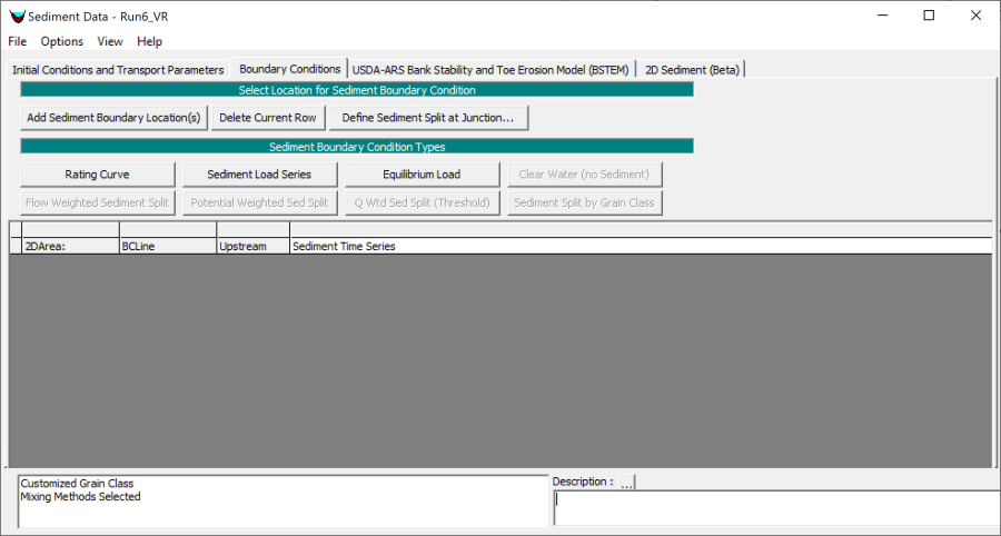
Figure 1. Boundary Conditions tab in the Sediment Data editor.

Rating Curve

The rating curve specifies the sediment load in tons/day or sediment concentration in mg/l as a function of flow discharge. The fractional composition of the incoming sediment load is specified for each grain class. The fractional loads are then specified to each cell using the cell sediment capacity as a weighting function. For 2D sediment transport, the user has the option to no specify the fractional bed-load composition. In this case, the cell sediment capacities (equilibrium concentrations) are used to compute the fractional sediment loads at each cell. This option is useful when the rating curve sediment gradations are not known.

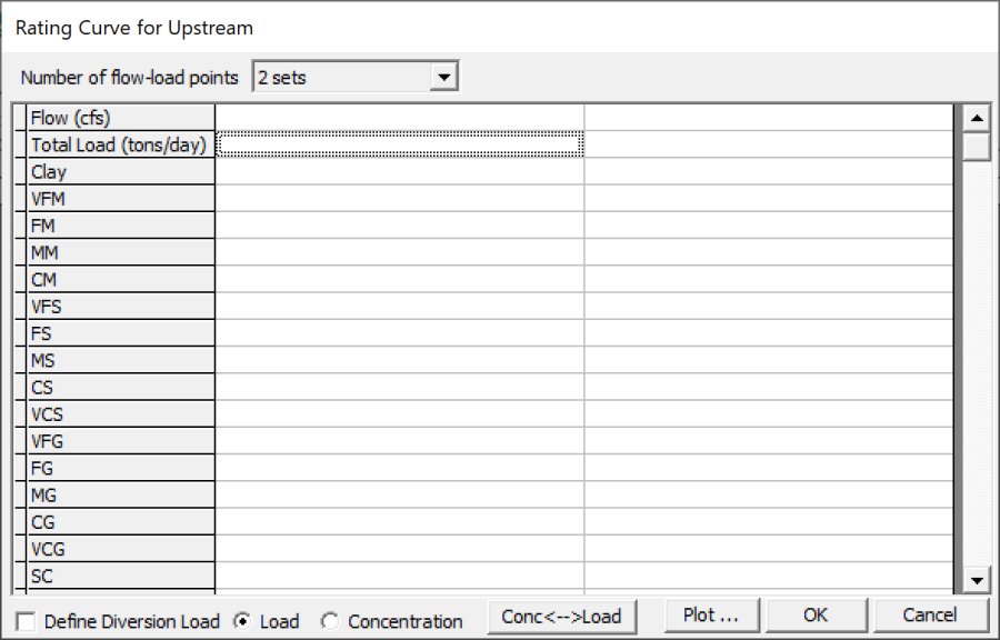
Figure 2. Sediment Rating Curve editor.

Sediment Load Series

The Sediment Load Series boundary condition specifies the sediment load in tons per time increment (see figure below). The sediment gradation may be specified with a Gradation Rating Curve or if this data is left empty, the gradation is determined by weighting the local (cell) equilibrium sediment loads. The Gradation Rating Curve specifies the gradation of the inflow sediment as a function of total load in tons/day. It is important to keep in mind that any grain specified in the gradation curve is automatically added to the computed grain classes.

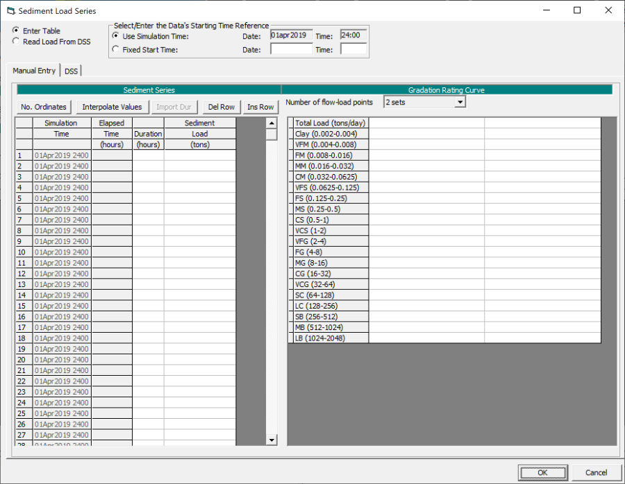
Figure 3. Sediment Load Series editor.

Equilibrium Load

The Equilibrium Load boundary condition specifies the inflow sediment load as the equilibrium sediment load. The equilibrium sediment load is computed as the equilibrium sediment concentrations at the boundary cells times the face flows. This approximation essentially assumes a zero-gradient concentration normal to the boundary. The equilibrium boundary condition should be used whenever data is not available or when first setting up a model in order to quickly get simulation results or to compare results from other boundary condition types which may be suspect.

Clear Water

The Clear Water boundary condition specifies a zero load/concentration at the boundary. This boundary is not very commonly used except for very specific situations.

Unsteady Temperature

Temperature is the only data the unsteady flow editor required for sediment transport analyses. Specify temperature for an unsteady sediment transport model in the Unsteady Flow Editor. Select the Water Temperature (for Unsteady Sediment)… option from the Options menu (see figure below).

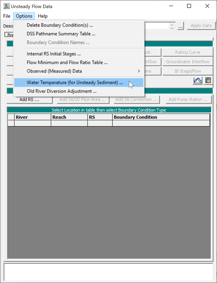
Figure 4. Opening the Unsteady Temperature editor from the Unsteady Flow Data editor.

The Unsteady Temperature time series editor, is similar to the unsteady flow and stage editors (see figure below). In the absence of temperature data in the unsteady flow file, HEC-RAS will assume 55.4ºF. The water temperature is used to compute the water kinematic and dynamic viscosities, and the water density which are then used by the sediment transport model.

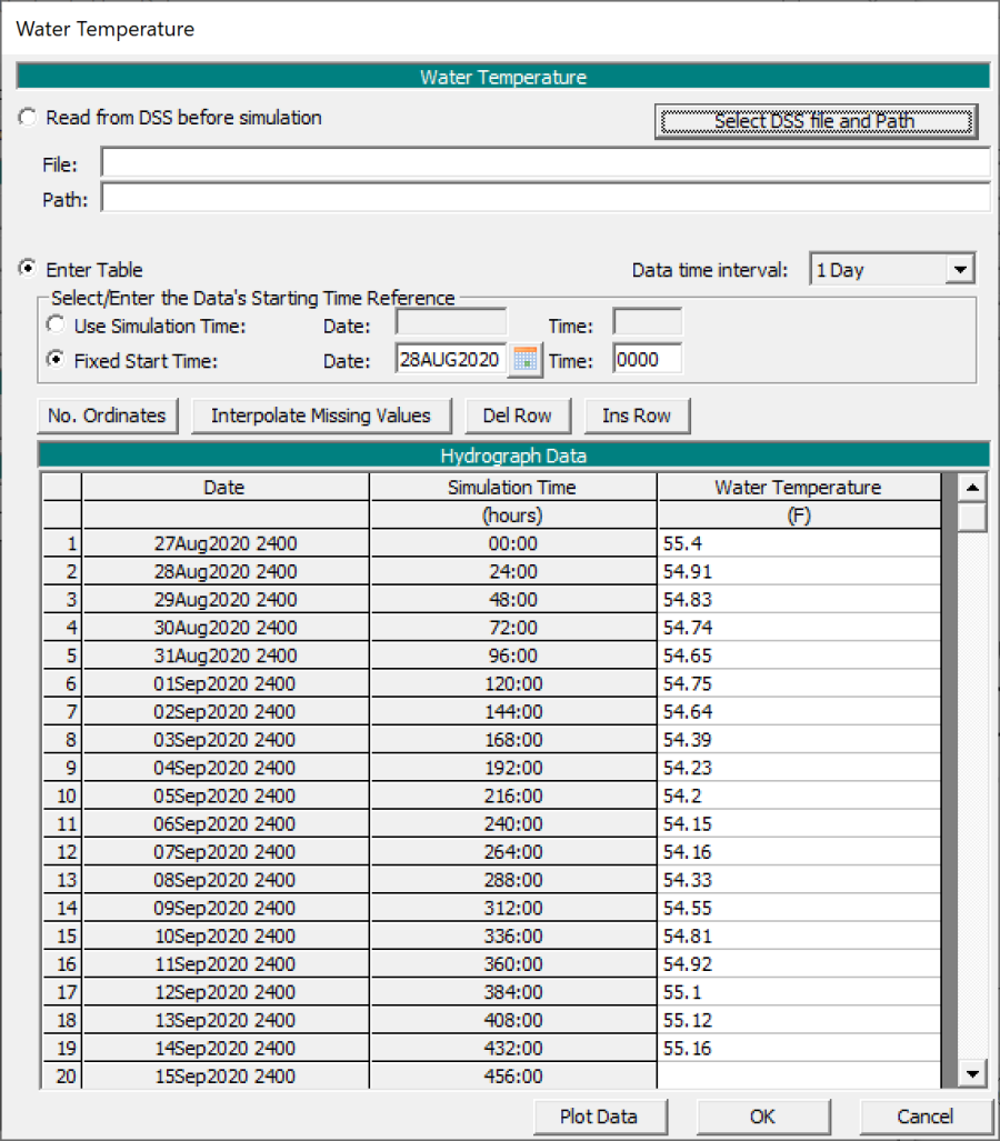
Figure 5. Specifying a temperature time series.