Download PDF
Download page Transport Methods.
Transport Methods
The Transport Methods editor is where the user may select the parameters and values for several transport-related variables. These include the Load Correction Factor, Diffusion Coefficient, and adaptation parameters. To open the Transport Methods editor, open the Sediment Data editor, and select open the Options menu and select Transport Methods… (see figure below).
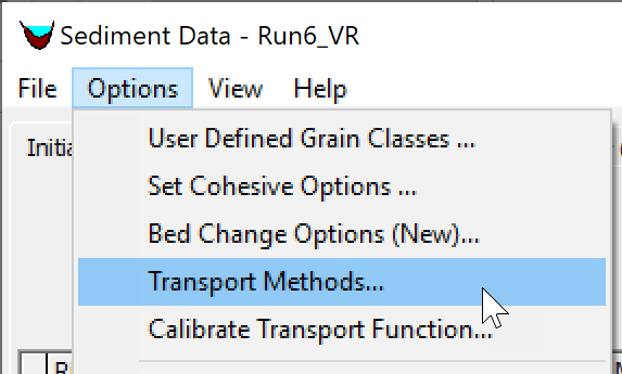
Figure 1. Opening the Transport Methods editor from the Sediment Data editor.
Load Correction Factor
HEC-RAS 2D sediment transport has the option to approximate the current velocity and concentration profiles with approximate semi-analytical profiles, as well as to utilize an empirical formula for the bed-load velocity (see figure below). If these options are enabled, a load correction factor is included in the temporal term of the transport equation (i.e. advection-diffusion equation). The load correction factor accounts for non-uniform vertical profiles of the concentration and current velocity as well as the bed-load velocity. Since most of the sediment concentration is typical near the bed where the current velocities are slower, the load correction factor is generally less than one and produces a temporal lag between the flow and the sediment concentrations.
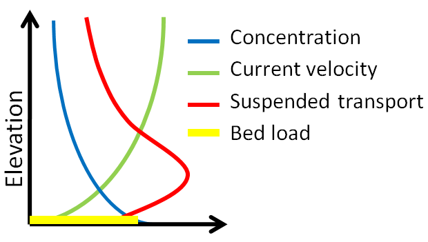
Figure 2. Schematic of sediment and current velocity profiles.
The load correction factor options are specified in the Transport Model and AD Parameters editor which can be accessed by opening the Sediment Data editor and selecting the menu Options and selecting Transport Methods…
The load correction factor options are specified within the section Total-Load Correction Factor section of the first tab of editor called AD Parameters. By default, HEC-RAS does not compute any load correction factors. To turn on the load correction factor the user may check the box labeled Total-load Correction Factor. One this checkbox is selected the user should select the methods used to compute the bed and suspended-load correction factors.
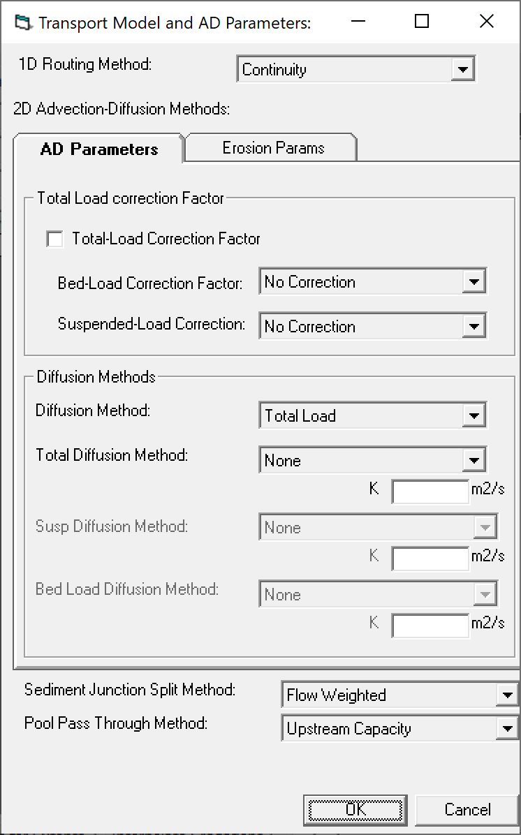
Figure 3. Setting the Total-load correction factor options in the Transport Model editor.
The bed-load correction factor method selects the formula for computing the bed-load velocity. The available bed-load velocity formulas are:
- No correction
- Van Rijn
- Van Rijn-Wu
- Phillips and Sutherland
Selecting No Correction assumes the bed-load velocity is equal to the depth-averaged velocity. The van Rijn and van Rijn-Wu are similar formulas. The only difference is that the van Rijn-Wu formula has coefficients that have been recalibrated with a larger dataset of measurements.
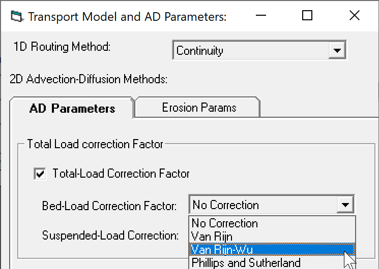
Figure 4. Setting the bed-load correction factor options in the Transport Model editor.
The suspended load correction factor methods select vertical sediment concentration profile. The three options are:
- No correction
- Rouse sediment concentration profile
- Exponential sediment concentration profile
When selecting the Rouse and Exponential sediment concentration profiles, it is assumed that the current velocity follows a logarithmic profile. If No Correction is selected, the suspended-load correction factor is set to one.
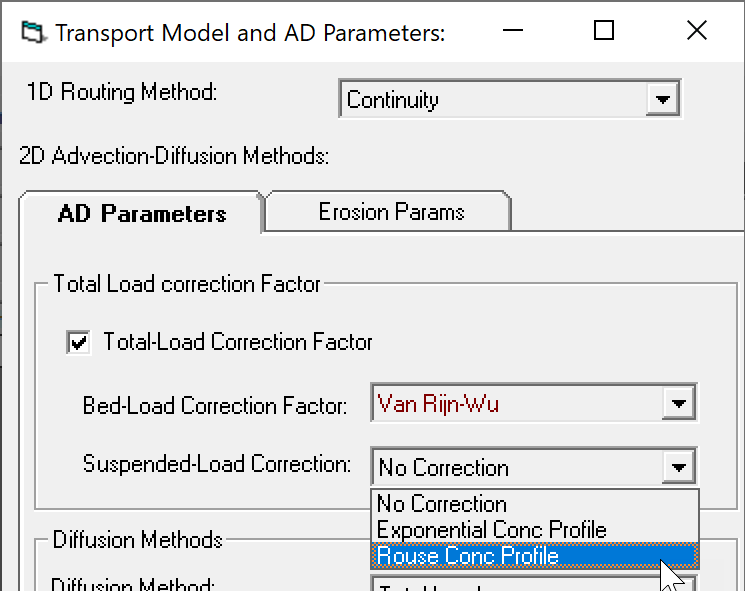
Figure 5. Setting the suspended-load correction factor method in the Transport Model editor.
Generally, for practical applications there is not enough data to calibrate the bed and suspended-load correction factors. Their use is a compromise between accuracy and computational time which are both relatively minor. In general, the morphology change is much more sensitive to other parameters and options such as the transport function and adaptation parameters than the load correction factors.
Diffusion Coefficient
Horizontal turbulent mixing and dispersion is modeled in HEC-RAS with a Fickian diffusion model. Turning on horizontal mixing is important in simulations with high resolution and sharp variations in sediment concentration capacities and concentrations, and when using high-resolution advection schemes. When the computational grid is relatively coarse or when using a first-order advection scheme the numerical diffusion may be so large that adding horizontal mixing is unnecessary. In general, sediment diffusion should not be used in combination with the Diffusion Wave Equation (DWE), since this can result and overly diffusive results.
The methods for computing the horizontal diffusion coefficients are in the AD Parameters tab of the Transport Model and AD Parameters editor which can be opened from the Sediment Data editor under Options and selecting Transport Methods... HEC-RAS has two options for the total-load diffusion coefficient.
- Constant
- Weighted bed-load and suspended-load diffusion coefficients
The default in HEC-RAS is for total-load diffusion of zero (i.e. no horizontal diffusion).
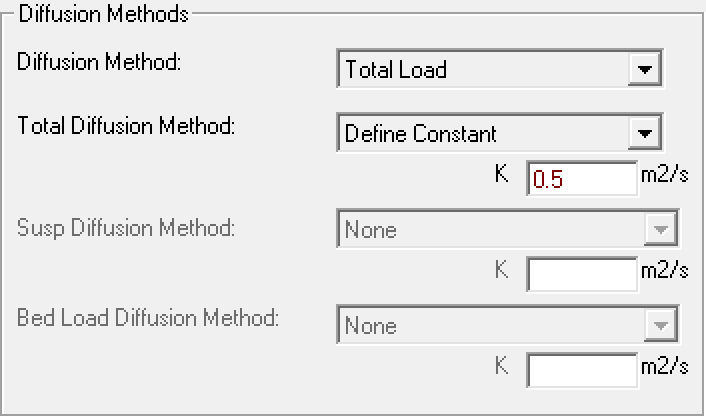
Figure 6. Specifying a constant total-load diffusion coefficient.

Figure 7. Specifying a total-load diffusion coefficient based on weighted bed and suspended load coefficients.
Erosion Parameters
The Erosion Parameters tab of the Transport Model and AD Parameters editor contains the settings for the noncohesive sediment transport erosion formulation. The total-load sediment erosion is computed as a function of the total-load adaptation coefficient. In HEC-RAS there are two methods for computing total-load adaptation coefficient:
- Total-load length
- Weighted bed-load and suspended-load adaptation coefficients
The total-load adaptation length computes the total-load adaptation length as a function of the unit discharge and sediment fall velocity (see figure below). The total-load adaptation length is the simplest and most computationally efficient of the two options.
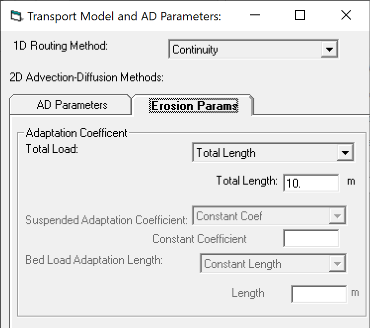
Figure 8. Specifying a total-load adaptation length.
The weighted bed-load and suspended adaptation coefficients requires specifying methods for the bed-load and suspended-load adaptation coefficients and computing the fraction of suspended sediments. However, it is the most physically accurate method.
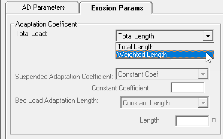
Figure 9. Specifying a weighted total-load adaptation length.
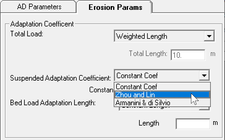
Figure 10. Specifying a suspended-load adaptation coefficient.
When first setting up a sediment transport model, it is recommended to use a constant total load adaptation length for simplicity. Once the user has a stable model producing reasonable results, it is recommended to perform a sensitivity of the adaptation length by adjusting the adaptation length. In many cases, the results are not found to be sensitive. This is usually for relatively coarse grid simulations under mild to moderate forcing. However, if the results are found to be sensitive to the adaptation length then more tests are necessary in determining to optimal adaptation method and parameters.