The Bed Mixing Options editor contains both 1D and 2D sediment bed mixing options and other parameters. The editor is opened from the Sediment Data editor by going to the Options menu and selecting Bed Mixing Options … (see figure below).

Figure: Accessing the Bed Mixing Options editor from the Sediment Data editor.

An example of the Bed Mixing Options editor is shown in the figure below. The sections which are applicable to 2D sediment are Hiding Functions and Active Layer Options.

Figure: Bed Mixing Options editor.

Hiding and Exposure Functions

HEC-RAS applies the transport functions to compute capacity for each grain class independently.  But coarse particles and finer particles do interact.  Finer (cohesionless) particles hide behind bigger particles and smaller particles collect below larger particles and raise (i.e. "expose") them into the flow field making them more transportable.  The hiding and exposure features reduce the transportability of the fine particles and increase the transportability of the coarse particles (relative to each other) to account for these processes.

If your model is over-predicting transport in the finer sand grain classes or under-predicting transport in the gravel and cobble grain classes, hiding and exposure can help.  The hiding (and exposure) function computes a correction to the incipient motion variable such as a shear stress or velocity to account for the hiding and exposure of particles. HEC-RAS has eight different hiding and exposure functions that are described in the technical reference manual here.

The hiding and exposure function can have a big impact on the results. Some of the hiding and exposure functions were developed for in conjunction with specific transport potential functions. For example, the Wu et al. (2000) hiding function was developed for use with bed- and suspended-load transport potential functions published in the same paper.  Because we often use the Wu transport function with 2D sediment, we often pair it with the Wu hiding and exposure function.  Similarly, the Day (1980) and Proffitt and Sutherland (1983) hiding function where developed specifically for the Ackers and White (1973) transport potential formula. Lastly the Wilcock and Crowe (2003) hiding function was developed specifically for the Wicock and Crowe formula (Wilcock 2001; Wilcock and Crowe 2003).

The following images illustrate how the exponent works in the Wu and Parker functions:

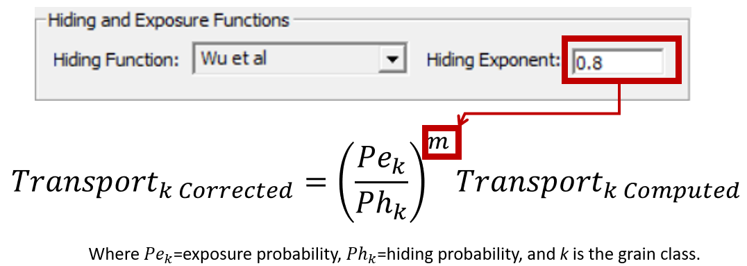
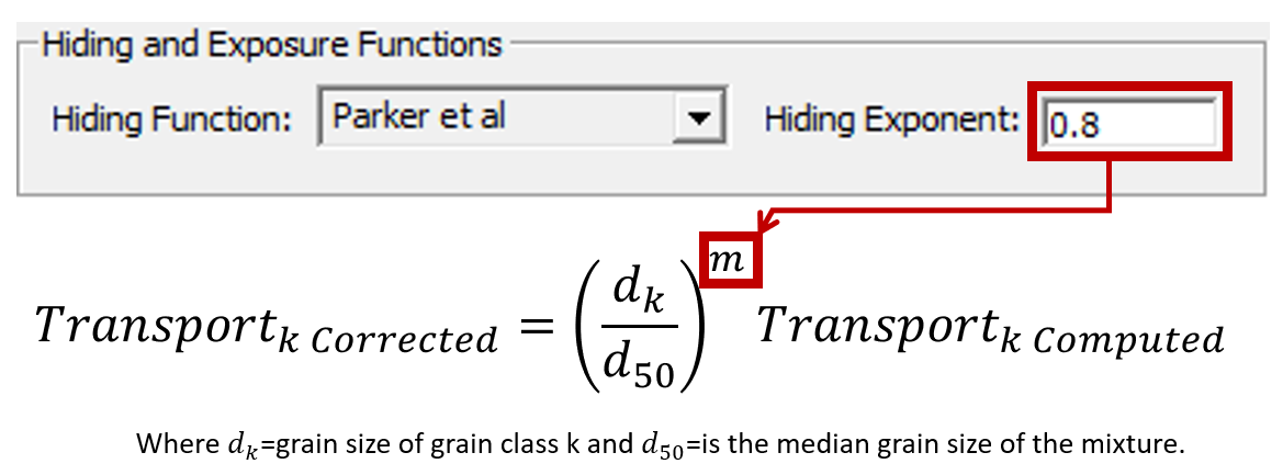
The exponent in the hiding and exposure algorithms can increase or decrease this effect.  An exponent of 1 exaggerates the hiding and exposure effects, actually making the cohesionless grain classes "equally mobile" (i.e. all grain classes have similar critical shear stresses).  An exponent approaching 0 mutes these effects (so that 0 essentially "turns off" the hiding and exposure effects).  

Hiding and Exposure tends to decrease transport but is the opposite of "armoring"

Hiding and exposure decreases the transport of finer particles and increases the transport of coarser particles.  But because transport is non-linear and finer particles are much more transportable, the bulk effect tends to reduce transport (less erosion, more deposition).  However, by decreasing the difference between fine and coarse particles, hiding and exposure also makes it more difficult for the model to coarsen the active layer to develop an "armor" layer.  So hiding and exposure can reduce the effectiveness of preconditioning runs, and increase erosion in select cases where an armor layer might form and reduce access to finer particles.

Note: The Hiding and Exposure notation can get complex

Note: The equation in the previous figure is a simplification of the more complex forms of the equations in the technical reference manual.  The hiding and exposure terms are often inverted, and then raised to a negative exponent.  For example, the transport corrected for hiding and correction () is related to the transport computed from the transport function () by a ratio such that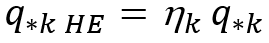.  But, is often inverted as such that the hiding and exposure function is raised to the negative exponent  making it, functionally, the equations describe above..  

The HEC-RAS default exponent (0.8) is not the recommended exponent for all equations.

HEC-RAS populates a default hiding exponent of 0.8.  But this is not the recommended exponent for all equations.  Wu, for example, recommends 0.6

Active Layer Options

Within the Active Layer Options section of the Bed Mixing Options editor are the input options controlling the active layer thickness and the Exchange Increment Method. The exchange increment is not utilized in the HEC-RAS 2D sediment transport model.

Active Layer Thickness

There are two methods for computing the active layer thickness: (1) d90, and (2) X d90. The  methods are selected within the Active Layer Options section of the Bed Mixing Options editor. The option d90 , the active layer is set to the 90th percentile diameter of the active times a user-specified multiplier. If the multiplier is set to 1, then the two methods produce the same results. 

One d90 is too small for sand models.

Active layers that are too small can limit erosion and affect model stability.  The one-to-three d90 paradigm of active layer thickness comes from the gravel bed transport literature where 2 d90s can be several inches to a foot.  But if your largest grain classes are sand, 1 to 5 d90's will be too small.  The default d90 is almost certainly too small.  Use a much larger multiplier here, and, preferably, also use a "Minimum Active Layer Thickness" (described below). 

Minimum Active Layer Thickness

The option is provided to specify a minimum active layer thickness within the Active Layer Options section of the Bed Mixing Options editor. This option is useful when simulating very fine material as the active layer thickness can become unreasonably small. Increasing the minimum active layer thickness may also reduce instability problems when the active layer gradation is changing very quickly.