The 2D Computational Options tab of the Sediment Computation Options and Tolerances editor contains the computational options which are utilized for 2D sediment transport (see figure below). The editor has options and parameters related to the subgrid erosion and deposition calculation methods, the advection scheme used in the transport solver, the matrix solver, outer loop convergence tolerances, the bed layer parameters, and subgrid options. 

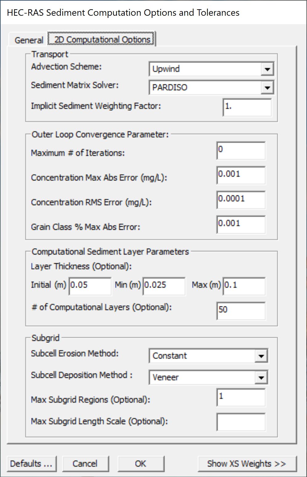
Figure 1. Specifying the warmup method for 2D simulations.

Subgrid Erosion and Deposition Methods

One of the key features of HEC-RAS 2D is the subgrid modeling. HEC-RAS 2D sediment has several methods for computing the subgrid erosion and deposition with different levels of complexity and computational requirements.
The erosion rate is computed as the erosion potential times the bed availability (grain fractions). Therefore, if the subgrid bed gradations vary, the subgrid erosion rates will also vary. However, the subgrid erosion potential may be calculated with one of four methods available (see table below).

Table 1. Summary of subcell erosion potential approaches.

The Constant erosion method is the simplest and most computationally efficient. For every cell, a single erosion potential is computed using wet-area averaged hydraulics, and bed properties. The bed properties include erosion coefficients, roughness, and grain size distribution, etc. The Depth-Weighted erosion method also computes a single erosion potential for every cell but applies a depth-weighting to compute the subgrid erosion potentials. Therefore, the Depth-Weighted method uses averaged bed and hydraulics to compute a cell erosion potential, but which is then weighted using the water depths to compute the subgrid erosion potentials. Again, subgrid erosion rates always take into account the subgrid grain fractions (material availability). The Depth-Weighted method is only slightly more computationally expensive than the Constant method. The Variable Bed erosion method does not perform depth-weighting but computes subgrid erosion potentials utilizing the subgrid bed properties. The Variable Bed method utilizes average hydraulic variables for the wetted area of the cell. The Full Subgrid erosion method does not perform depth-weighting but computes subgrid erosion potentials utilizing the subgrid bed properties and hydraulics. The method requires estimating subgrid hydraulic variables such as current velocities, shear stresses, shear velocities, depths, etc. depending on the transport potential formula utilized. The Full Subgrid method is the most computationally expensive of all the methods and will generally lead to the largest variations in subgrid erosion compared to the other methods. All of the erosion methods assume that a constant adaptation coefficient within the cell.
HEC-RAS 2D sediment has three subgrid deposition methods (see table below). All the deposition methods assume that the sediment concentration and adaptation coefficient are constant within a cell. The first is the Veneer method. The Veneer method applies a spatially constant deposition rate over the wet portion of the cell. The Veneer method is the simplest and most computationally efficient of the methods. The Veneer deposition method is analogous to the Veneer method utilized in HEC-RAS 1D sediment transport. The Depth-Weighted deposition method is similar to the Reservoir method in HEC-RAS 1D sediment transport. The Capacity-Weighted deposition method is similar to the Capacity-Weighted erosion method.

Table 2. Summary of subcell deposition approaches. 

Advection Scheme

HEC-RAS 2D sediment transport has the option to choose between four advection schemes:

1. Upwind
2. Exponential
3. Minmod
4. Harmonic

The selected advection schemes are designed to off the use a wide range of options. The Upwind and Exponential schemes are first-order difference schemes (Patankar 1980). The schemes are linear and therefore have the benefit of not requiring additional outer loop iterations. In addition, difference schemes are relatively simple, and provide smooth bounded solutions. The Exponential scheme is based on the analytical solution of the steady 1D advection-diffusion equation (without sources and sinks) and is less diffusive than the Upwind scheme. However, when the horizontal mixing is turned off, the Exponential scheme reduces to the Upwind scheme.
The Minmod and Harmonic schemes are high-resolution Total Variance Diminishing (TVD) schemes (Harten 1983). High-resolution TVD schemes allow for second order or higher accuracy in smooth and first-order accuracy in sharply varying regions without producing spurious oscillations (bounded solutions). The TVD schemes are implemented here using a flux-limiter formulation and a deferred correction approach which requires outer loop iterations to converge. The Minmod scheme has good convergence characteristics but is the most diffusive of the two TVD schemes. The Harmonic scheme is less diffusive, produces good convergence characteristics in implicit schemes, and is equivalent to the Hybrid Linear/Parabolic Approximation (HLPA) scheme of Zhu (1992).

Matrix Solvers

HEC-RAS 2D Sediment Transport solves an implicit Advection-Diffusion (transport) equation for the fractional total-load concentrations. The discretization produces a linear system of equations which may be represented by a sparse-matrix problem. The sparse matrix solver is an important component of the computational options because a large portion of the computational time can be spent solving the sparse matrices for each grain class transport equation. HEC-RAS has three options for the matrix solver:

1. PARDISO
2. FGMRES-SOR
3. FGMRES-ILU0

The PARDISO solver is a high-performance, robust, memory efficient and easy to use solver for solving large sparse symmetric and non-symmetric linear systems of equations on shared memory and distributed-memory architectures. Here the Intel Math Kernel Libraries (MKL) PARDISO solver is utilized. The solver utilizes a combination of parallel left- and right-looking supernode pivoting techniques to improve its factorization process (Schenk et al. 2004; Schenk et al. 2011).
Iterative solvers require an initial guess to the solution. Iterative solvers generally require less memory for because unlike with direct solvers, the structure of the matrix does not change during the iteration process. In addition, iterative solvers utilize matrix-vector multiplications which can be efficiently parallelized. The main drawback of iterative solvers is that the rate of convergence depends greatly on the condition number of the coefficient matrix. For poorly conditioned matrices, the iterative solver may not converge at all. Therefore, the efficiency of iterative solvers greatly depends on the size and condition number of the coefficient matrix.
Iterative solvers may be classified into stationary and projection methods. In stationary methods the solution for each iteration is expressed as finding a stationary point for the iteration. The number of operations for iteration step for stationary methods is always the same. Stationary methods work well for small problems but generally converge slowly for large problems. Projection methods extract an approximate solution from a subspace. Generally, projection methods have better convergence properties than stationary methods but because each iteration is generally more computationally demanding than stationary methods, they tend to be more efficient for medium to large systems of equations. The main disadvantage of iterative solvers is their lack of robustness.
HEC-RAS 2D sediment has the option of two iterative solvers: FGMRES-SOR and FGMRES-ILU0. The first part FGMRES refers to the matrix solver while second parts SOR and ILU0 refer to the preconditioner utilized. FGMRES (Flexible Generalized Minimal RESidual) is a projection method which is applicable to coefficient matrices which are non-symmetric indefinite (Saad, 1993). The "flexible" variant of the Generalized Minimal RESidual method (GMRES) allows for the preconditioner to vary from iteration to iteration. The flexible variant requires more memory than the standard version, but the extra memory is worth the cost since any iterative method can be used as a preconditioner. For example, the SOR could be used as a preconditioner with different relaxation parameter values each time it is applied. The FGMRES (and GMRES) method becomes impractical for large number of iterations because memory and computational requirements increase linearly as the number iterations increases. To remediate this the algorithm is restarted after iterations with the last solution used as an initial guess to the new iterative solution. This procedure is repeated until convergence is achieved. The FGMRES solver with restart is often referred to as FGMRES(m) where m is the restart parameter. However, here the shorter name FGMRES is used for simplicity. If m is too small, the solver may converge too slowly are even fail completely. A value of m that is larger than necessary involves excessive work and memory storage. Typical restart values are between 5 and 20. Here m is set to 10 which works well for the most practical applications.
The Successive-Over-Relaxation (SOR) is a stationary iteration method based on the Gauss-Seidel (GS) method. When ω = 1, the SOR method reduces to the Gauss-Seidel method. In addition, for ω < 1, the method technically applies under-relaxation and not over-relaxation. However, for simplicity and convenience the method is referred to as SOR for all values of ω. Kahan (1958) showed that the SOR method is unstable for relaxation values outside of 0 < ω < 2. The optimal value of the relaxation factor is problem specific. The SOR method is guaranteed to converge if either (1) if 0 < ω < 2, and (2) the matrix is symmetric positive-definite, or strictly or irreducibly diagonally dominant. However, the method sometimes converges even if the second condition is not satisfied. For simplicity, the relaxation parameter is set to 1.3 here and cannot be adjusted by the user. The value of 1.3 has been found to work reasonably well for a wide range of problems. A simple parallel version of the SOR is utilized here which is referred to as the Asynchronous SOR (ASOR) which uses new values of unknowns in each iteration/updates as soon as they are computed in the same iteration (see Chazan and Miranker 1969; Leone and Mangasarian 1988). The ASOR is part of a class of iterative solvers known as chaotic relaxation methods. Since the order of relaxation is unconstrained, synchronization is avoided at all stages of the solution. However, the convergence behavior can be slightly different for different number of threads. The ASOR solver has been parallelized with OpenMP.
The SOR preconditioner is based on the SOR solver except that no convergence checking is done during the iteration process (DeLong 1997). This is done for simplicity and to avoid additional computations associated with the determining the convergence status. The SOR preconditioner is utilized for non-symmetric matrices. The SOR preconditioner matrix is given by
The ILU0 (Incomplete Lower Upper with Zero Infilling) is part of a large class of preconditioners which utilize incomplete factorizations of the coefficient matrix. The effectiveness of the preconditioner depends on how well the sparse matrix by factored into lower and upper sparse matrices. ILU0 is one of the most common types of incomplete factorizations. In this factorization, all non-zero values of the exact factorization which are located in zero value positions are discarded. The advantage of the ILU0 preconditioner is that it preserves the structure of the original matrix. Another advantage of ILU0 versus other similar factorizations is that it does not require specifying additional tolerances and settings.

Outer Loop Convergence Options

The outer loop refers to the loop in which the transport equations are coupled to the bed change and sorting equations whereas the inner loop is the iterative solver loop. The outer loop is also necessary for updating the deferred corrections from the high-resolution advection schemes. If a direct sparse matrix solver is utilized, there is no inner loop. The maximum number of outer loop iterations may be set by user (see figure below). The maximum number of outer loop iterations is a compromise between computational efficiency and accuracy. If the sediment model is iterating every time step and going to the maximum number of iterations, this is an indication, the either the time step is too big or the convergence tolerances have been set too small. Outer loop convergence is monitored by change in the sediment concentrations and active layer bed fractions between outer loop iterations. The convergence of the fractional total-load sediment concentrations is assessed by means of two tolerances. The first is the maximum value of the absolute differences (errors) in concentrations between outer loop iterations. The second is the root-mean-square of the differences (errors) between outer loop iterations. For the first iteration, the error is approximated by comparing the current concentrations with the previous time step values. The convergence of the active bed grain fractions is assessed by means of a maximum absolute error tolerance. This approach works well for both constant density and variable density simulations.

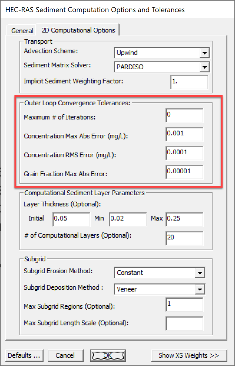
Figure 2. Outer loop Convergence Parameters.

Whenever, the sediment concentrations or active layer grain fractions do not converge or reach the maximum number of iterations, a message is printed to the log file. In addition, the convergence status is written to the HDF5 file at the Mapping Output Interval. This log information can be used to optimize the convergence parameters and computational time step.
When simulating Non-erodible Surfaces, the active layer grain fractions can vary significantly in a time step and even within a time step (outer-loop iterations). Therefore, it is expected that when simulating Non-erodible Surfaces with multiple-grain classes, at least one or two iterations will be needed for the active layer fractions to converge. In fact, even when simulating a single grain class, iterations are still required because for the sediment concentrations to convergence above Non-erodible Surfaces because the erosion rates are limited before solving concentrations using an expression which includes an estimate of the deposition rates from the previous iteration.

Computational Sediment Layer Parameters

There are two types of layers in HEC-RAS. The first type is the bed layers which are used to specify the bed gradations and the second is the computational bed layers which are used in the solution of the bed sorting and layering. Specifying initial sediment bed layers is optional. If the user does not specify initial bed layers, a vertically uniform bed composition is assumed, and computational bed layers are created based on the user-specified initial bed layer thickness (see figure below).

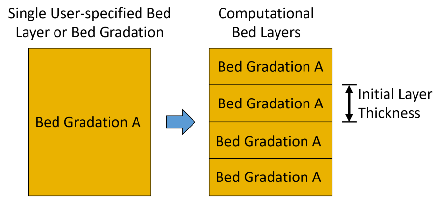
Figure 3. Calculation of computational bed layer thickness from a single user-specified initial bed layer or bed gradation.

If the user specifies initial bed layers, these are subdivided (discretized) such that the initial bed layer thickness is equal to or less than then the user-specified initial bed layer thickness (see figure below).

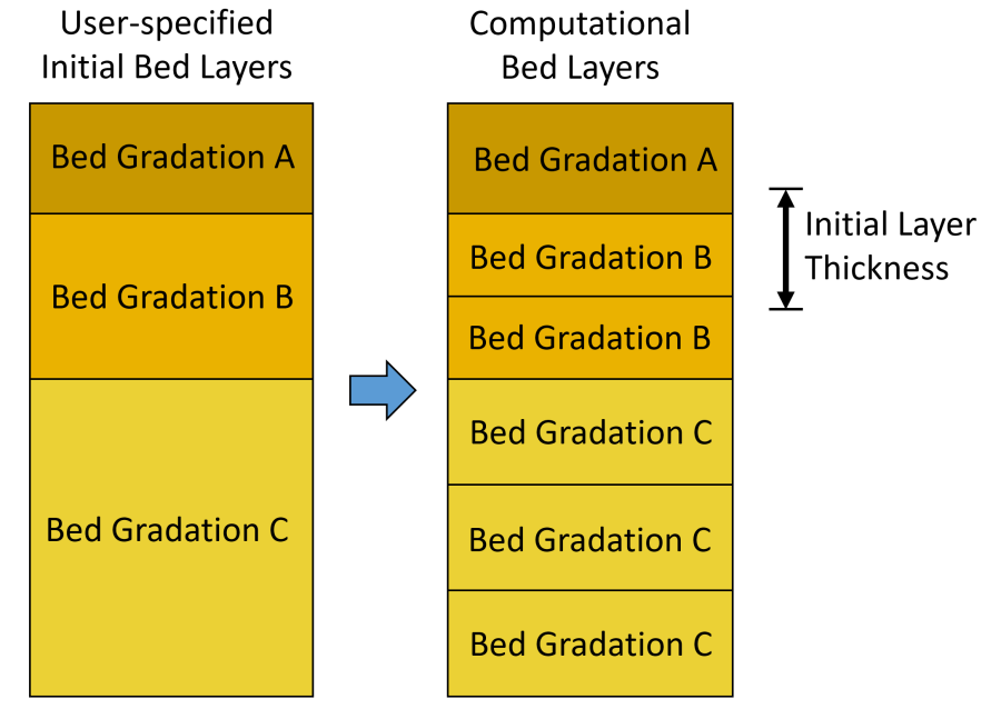
Figure 4. Calculation of computational bed layer thickness and composition from user-specified initial bed layers.

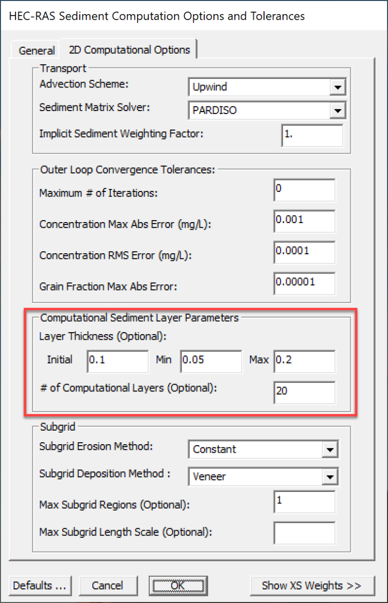
Figure 5. Computational Sediment Layer Parameters section in the HEC-RAS Sediment Computation Options and Tolerances editor.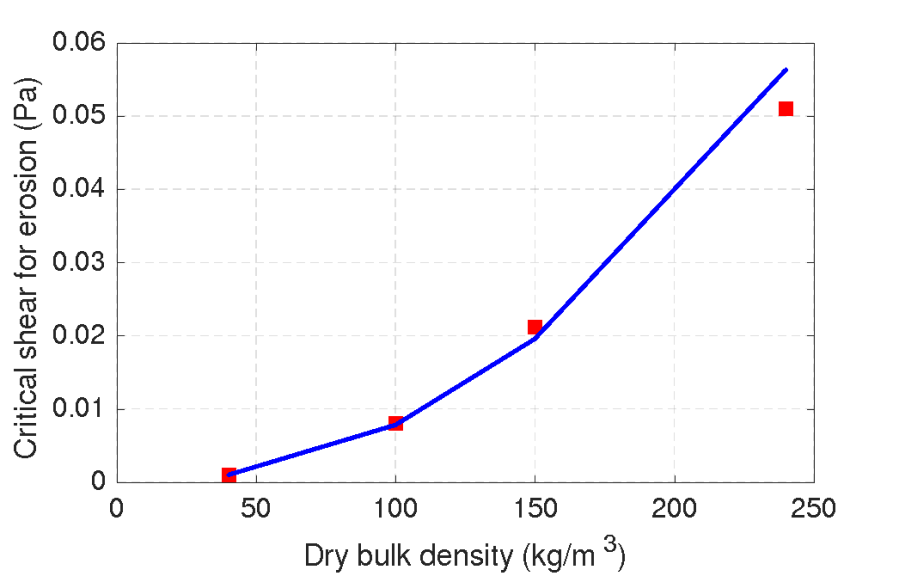



Figure 6. Example of a power-law parameterization of the critical shear for erosion as a function of the dry bulk density.