Most of the sediment transport equations were developed with sand and/or gravel data. Therefore, most silt and all clay particles are outside of the range of applicability of the sediment transport functions implemented in HEC-RAS. In most systems, these particles are wash load, material only found in the bed in trace amounts, because transport capacity always exceeds supply. Some modelers will just ignore fines as throughput load, arguing that if fines never interact with the bed in the model reach, the model is insensitive to them and they add unnecessary complexity and parameters to the model. However, sometimes fines must be modeled explicitly. In reservoirs and other backwater or low energy zones, silt and clay can deposit and clay lined channels, both natural and engineered, can erode, causing local and downstream problems.
Fine sediment transport is further complicated by electrostatic and electrochemical forces. These particles are not just outside of the empirical range of the equations, but they often erode and deposit by fundamentally different processes. These forces cause fine particles, particularly clay, to flocculate and "stick" to the bed surface, so that fine erosion and deposition are often not primarily functions of sediment size. These processes make fine deposition and erosion fundamentally different than the cohesionless sand and gravel transport.
In HEC-RAS, the cohesive options can be set by selecting Set Cohesive Options… under Options menu of the Sediment Data editor (see figure below).

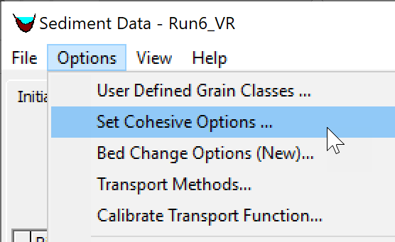
Figure 1. Opening the Cohesive Options editor from the Sediment Data editor.

The Cohesive Options editor is shown in the figure below. The editor allows the user to select how the erosion is computed for cohesive sediments.

Erosion Parameters

HEC-RAS includes three cohesive erosion methods; applying the standard transport equations, or two different implementations of the Krone and Partheniades approach. In HEC-RAS 2D sediment transport, the HEC 6T Capacity Method is not available. When utilizing the 2D sediment transport model, it is generally not recommended to use the transport functions for the cohesive grain classes, especially clay. If the cohesive grain classes represent a very small fraction of the bed gradation, then it is better to simply remove them from the bed gradation then it is better to model them as cohesive.

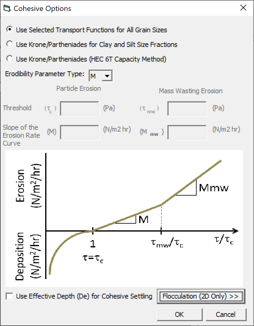
Figure 2. Cohesive Options editor.

The treatment of cohesive sediments and mixtures of cohesive and noncohesive sediments is slightly different for HEC-RAS 1D and 2D. HEC-RAS 1D considers the smallest five grain classes 'fine sediment'. HEC-RAS 1D applies the same cohesive erosion method selected to these grain classes. By default, the first five grain classes are the clay and silt classes, and are all finer than 0.0625 mm. However, if the user edits the diameters sizes for these, the cohesive erosion methods will still apply to the first five grain classes, regardless of their size. HEC-RAS 2D has diameter thresholds that determine whether a grain class forms flocs and behaves cohesively on the bed. The reason for having these separate thresholds is to allow for the erosion to be calculated with the user-selected transport function while still allowing fine grain classes to form flocs. The upper threshold for grain classes to form flocs is 0.0625 mm. The size tolerance for grain classes are behave cohesively on the bed is either set to 0.0 mm if the Use Selected Transport Functions for All Grain Sizes option is selected or 0.0625 mm if the Krone/Partheniades formulas are selected.
In HEC-RAS 1D if more than 20% of the active layer is cohesive, then the model considers the sediment active layer as cohesive and computes the erosion for all grain classes using the cohesive method. However, in 2D the erosion of mixed cohesive/noncohesive sediments is computed
Ariathurai (1974) parameterized Partheniades (1962) results into a formula with an erosion rate coefficient M and critical shear for erosion τc. M and τc include the stochastic nature of both the sediment bed composition and surface and the bed shear stress. The critical shear for erosion is usually in the range of 0.2 to 0.8 Pa, while M is usually in the range widely from 0.01 to 50 Pa/hr (Winterwerp and van Kesteren 2004). Dahl et al. (2018) obtained good results in simulating the lower Mississippi river using τc = 0.02 lb/ft², τmw = 0.04 lb/ft², M = 0.05 lb/ft²/hr, and M = 0.03 lb/ft²/hr.

Flocculation

The settling velocity of cohesive particles is computed using a flocculation settling velocity. The flocculation settling velocity takes into account the formation and destruction of flocs as a function of the sediment concentration. HEC-RAS has two methods for estimating the settling velocity of flocs (see figure below). The first is the method of Hwang (1989). The method represents the settling velocity as 4 separate zones: (1) free settling, (2) flocculation, (3) hindered settling, and (4) negligible settling. The method requires 4 empirical coefficients.

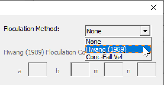
Figure 3. Selecting the Hwang (1989) floc settling velocity formula.

Example coefficient values for the Hwang (1989) formula are shown in the table below.

Table 1. Example coefficient values for the Hwang (1989) formula from literature.

The second method available to estimate the floc settling velocity is a user-specified Flocculation Curve. The Flocculation Curve defines the settling velocity as a function of the suspended sediment concentration. An example of a user-specified flocculation curve is shown in the figure below. The free-particle settling velocity is used when it is higher than the user-specified fall velocity for concentrations less than the concentration at the peak settling velocity. When the concentration is high than the maximum concentration specified in the flocculation curve, the settling velocity corresponding to the maximum concentration is used.

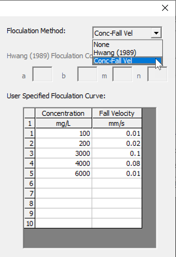
Figure 4. Specifying a floc settling velocity as a function of suspended sediment concentration.

In addition to taking into account the sediment concentration, HEC-RAS corrects the floc settling velocity for the water temperature by applying a correction which is a function of the water dynamic viscosity. This assumes that the user-specified curve and the coefficients in the Hwang method correspond to a standard water temperature of 55.4ºF.

Consolidation

Consolidation curves are developed for a specific bed material. Since HEC-RAS only allows the user to specify one consolidation curve, a representative consolidation curve is used for the all of the modeling domain. It is assumed that the consolidation curve was developed for cohesive sediments. Until more than one consolidation curve is added to HEC-RAS a simple correction is computed to account for the presence of noncohesive sediments which can significantly affect the consolidation curve.

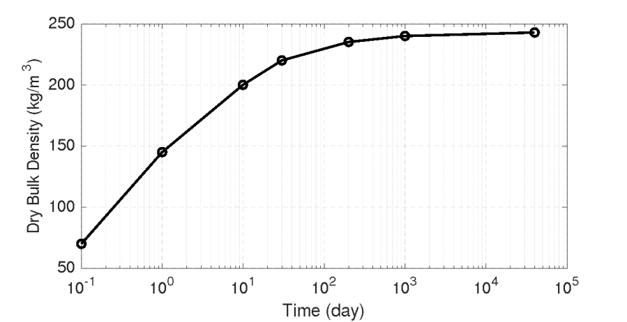
Figure 5. Example consolidation curve of dry bulk density as a function of time.