Download PDF
Download page Creating an Combined 1D/2D Model.
Creating an Combined 1D/2D Model
This document describes the basic steps in creating an combined 1D/2D river hydraulics model in HEC-RAS. Steps for creating, refining, reviewing, and comparing to alternative plans will be discussed. This document will not provide the level of detail that you can get from the HEC-RAS User's Manual, HEC-RAS 2D User's Manual, or the HEC-RAS Mapper User's Manual and should be considered a guiding document for typical or general steps, guidance, and problems you might encounter in building and refining an HEC-RAS model.
Create a New Project
Before you can start building an HEC-RAS model, you need to create a new project. Choose the File | New Project menu item on the main RAS interface, as shown below.

Provide a name (and filename for the project).

A window will informed you of the unit system to be used for the project.

All project files will begin with the file name. In the example above, the model title is "Combined 1D/2D Model" and the project filename is "Combined.prj". When I create new data files (geometry, flow, plan, ...) the project name will be appended with with a suffix corresponding an enumeration for the type of file that is created.
So for this example, the following files will be created for the first of it's type.
- Project File - Combined.prj
- Geometry File - Combined.g01
- Steady Flow File - Combined.f01
- Unsteady Flow File - Combined.u01
- Plan File - Combined.p01
A Plan is similar to an alternative and will be comprise of a geometry file and a flow file. A visual chart of the plan and file structure for HEC-RAS is shown below.

Base Project Data
RAS Mapper will be used to create the geometry for the HEC-RAS model. Click the RAS Mapper button from the main RAS interface.

Projection
Set the coordinate system for the project. The projection will be used to reproject any data that is brought into RAS Mapper. This include terrain data and land cover data when you create new datasets or background data such as shapefiles and web imagery. To set the projection, choose the Project | Set Projection menu item.

Select the Browse folder button to select an esri PRJ file. If GDAL doesn't recognize the projection, you will be provided a warning message.

Terrain
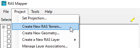
A good HEC-RAS model requires good terrain data. Especially when it comes to a 2D model as it is much more difficult to supplement data in a 2D model compared with a 1D cross sections. To begin using ground elevation data in HEC-RAS, select the Project | Create New RAS Terrain menu item in RAS Mapper.
Select the terrain model(s) of interest. Specify the parameters for the new RAS Terrain (rounding, vertical conversion) and provide a unique filename.

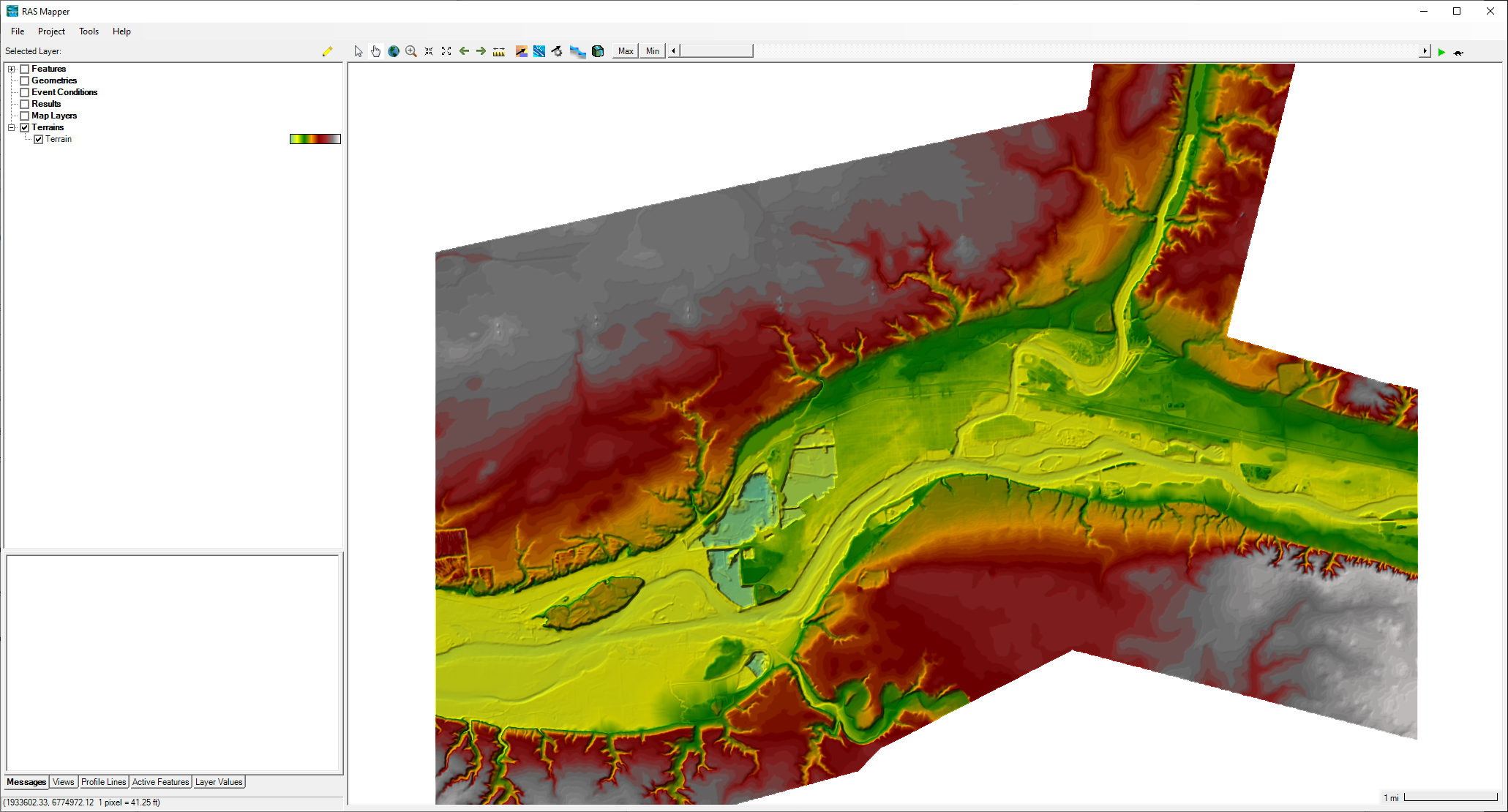
Click the Create button. RAS Mapper will effectively import the terrain data (it creates a copy from the input dataset) based on the specified parameters. During the import process, the data will be rounded, converted, tiled (for zoom levels), and re-projected (if necessary) to the coordinate system specified.

When complete, there will be new files created on disk: a Terrain.hdf file that contain information RAS Mapper uses to manage the terrain data, a Terrain.vrt file that can be used to visualize the terrain data in other programs, and a Terrain.Tif for the data that was imported (multiple .tif files will be created if the user specified multiple inputs). The Terrain.hdf file will then be loaded into RAS Mapper for visualization and use.
Land Cover Data
If you have a land cover datasets for use with Manning's n values, that might be the next thing you prepare for modeling. To import a land cover dataset, select Project | Create a New RAS Layer | Land Cover Layer.

Add the land cover layers of interest. At this time, you can re-classify the data if desired. Enter a cell size for new raster that is created and provide a unique filename. Click Create to create a byte raster (integer grid) of land cover data.

The data import will create a LandCover.hdf file for use in RAS Mapper and a LandCover.tif which holds the classification information. Once the data has been imported, it will be added to the map display in RAS Mapper.

Set Manning's n Values
To assign Manning's n Values to the land cover dataset, right-click on the land cover dataset and choose the Edit Land Cover Data Table.

The Classification Parameters table will open and allow you to enter an n value for each classification type.

Classification Polygons
Land cover data can be refined using vector data on the land cover raster. The Classification Polygons are included as a child layer and can be used to reclassify the land cover data for areas where you wish to have more detailed data, such as the channel.
Create a New Geometry
In RAS Mapper, select the Project | Create New Geometry menu item.

Provide a unique name for the geometry.

Press OK to create a new Geometry and add iit to RAS Mapper. Layers without data are shown in grey and as you create data the layer names will turn black and the layer's symbology will be shown.

Once a Geometry has been added, it can then be place in editing mode to start creating model geometry.
Associate Base Data
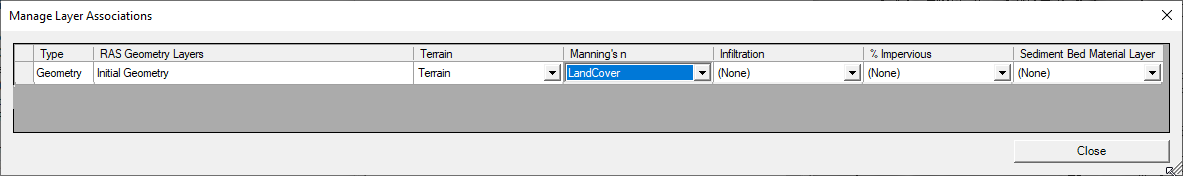
Before you start creating model geometer, you need to associate the Terrain layer and the Land Cover layer with the Geometry. Select the Project | Manage Associations menu item.

Associate the Terrain and the Manning's n dataset in the dialog that is provided. Press the Close button when finished.
Options
There are several options available from within RAS Mapper to customize the data extraction and visualization. Access the Options from the Tools | Options menu item.

From the Option dialog you can set River Station unit system, elevation point filtering, RAS Layer symbology, Editing Tools, and many others.

Create a 1D Geometry
The first step in creating any steady or unsteady model is to create a steady, 1D model to get an understanding of the river system. Start creating the combined 1D/2D model by Editing the initial Geometry.
To start editing a geometry, select the Geometry layer of interest an click the Start Editing button (this button will be replaced with the Stop Editing button).

River
The first thing to create in a 1D model, is to digitize the river system. The River Layer is used to hold the river system. Select the Rivers Layer, and using the Add New Feature tool, create a river centerline. River centerlines are created from upstream to downstream through the main portion of the channel. To finish creating a river line, double-click the polyline. This will close the line and invoke the River and Reach Name dialog. Provide a unique river and reach name.

To add a another river, such a tributary, create another river reach.
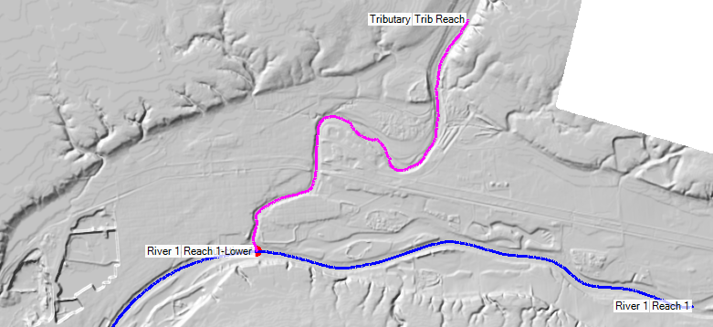
Double-click to end the tributary on the main river. If you are close to the original river (look for the red circle at the end of the river reach), you will be asked to create a junction. In RAS, a junction signifies a location to combine (or split) flow. The steps in creating a junction are listed below.
- Split the original river

- Rename the new river reach

- Provide a junction name

Junction information should be edited from the Geometric Schematic. Verify that the junctions lengths are appropriate and the desired modeling method is selected.
Bank Lines
Bank Lines are used to identify the main channel conveyance from the the overbanks. Create a bank line for the left and right overbanks for each river. The bank lines will also be used for creating an Interpolation Surface that is used for mapping results. Therefore, be careful to place the bank line as precisely as possible for where flow separation from the main channel and overbanks will occur. It is often helpful to use aerial imagery to assist in locating bank lines. Obviously, refinement of this layer will be necessary as you gain insight into the river system. Example bank lines are shown in the figure below.

Flow Path Lines
Flow Path Lines are used to compute the reach lengths for the left and right overbank. The River Lines will be used to compute the reach length in the main channel. The flow path lines should follow the center-of-mass of flow in the overbank.
Cross Sections
For the 1D portions of the model create cross sections covering the entire floodplain for the range of flows to be modeled. Cross sections should be located so that they capture controlling locations along the river as well as being created close enough together to smoothly capture the changes in terrain. A handy, back of the envelop, way to think about it is that no cross section should be no farther away that how wide it is. Cross sections should be constructed in the main channel and overbanks such that they are dog-legged perpendicular to flow. Having the bank lines and flow path lines available will assist in properly laying out cross sections.
Before laying out cross sections, be sure to set the River Station units for "numbering" the cross sections. The default units are feet/meters but for large river you should choose miles/kilometers. As you layout cross sections, RAS will compute the river station for the cross section and make the river station unique. So if you place the cross sections close together, RAS Mapper will keep incrementing the number of decimal places until the river station differs from its neighbor.
Another helpful option in RAS Mapper is to turn on the Contour Lines on the Terrain layer. The image below shows the location of cross sections on the Terrain with the river line, bank line, and contour lines.

If you want preview what the cross section will look like, use the the Cross Section Plot tool. The cross section will update each time you update a point on the cross section.

As you lay out and edit cross section locations, data will automatically be extracted. By default, River Stations will be plotted at the start of each cross section. Additional Plot Options available for the cross sections are accessed on the Layer Properties.

Additional Data
There are a multitude of addition 1D data you might want to create, from Ineffective Flow Areas, Blocked Obstructions, Bridges, Inline Structure, and Storage Areas. We will skip these data at this time.
Geometric Data Editor
When finished creating data in RAS Mapper, Stop Editing and close RAS Mapper.
Open the Geometric Data Editor from the main HEC-RAS interface.

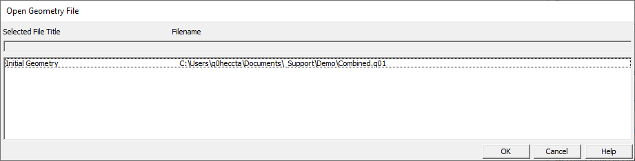
Load the Geometry by selecting File | Open Geometry Data.

Select the geometry you were working on in RAS Mapper.
You may need to complete some of the geometry such as Manning's n values, filtering cross section points, adding ineffective flow areas, etc.

When you have finished making obvious edits, close the Geometric Data Editor.
Create 1D Steady Flow Data
Open the Steady Flow Data Editor from the main HEC-RAS interface. Enter flow data for the range of flows you expect to model. Depending on the river system, entering a low flow like the 2-year flow can help identify the main channel and verify the location of bank stations. Entering a high flow will help you identify the entire floodplain and verify the cross section extents.

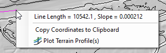
Next, enter a downstream boundary condition. Normal depth is a quick way to enter a boundary condition. Of course, you should have extended the downstream portion of the model downstream of the main area of interest and selected a highly 1-dimensional portion of the river. First, figure out the general slope of the river. This can be done in RAS Mapper, but selecting the measure Measure Tool and digitizing a portion of the river. After double-clicking to end the draw, the slope will be reported.
Enter the Normal Depth Slope but click on the cell for the downstream boundary of the river and clicking the Normal Depth button.

Save the flow data before moving to on to create a steady flow plan.

Create 1D Steady Flow Plan
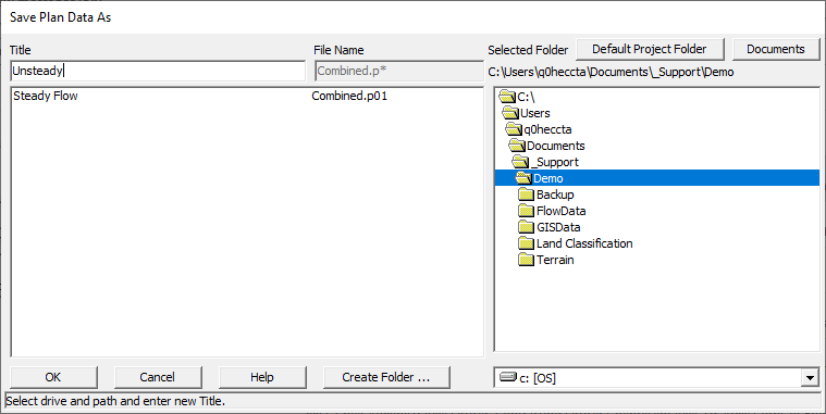
In order to run the HEC-RAS model, create a Steady Flow plan using the initial geometry and steady flow data. From the Steady Flow Analysis window, select Save Plan and provide a plan name. You will also be prompted for a Short ID which is used for labeling output plots.


Once a plan is created, you are ready to compute hydraulic results.

Compute water surface profiles by clicking the Compute button. Provided data has been adequately entered, the interface will provide status messaging during the steady flow run.
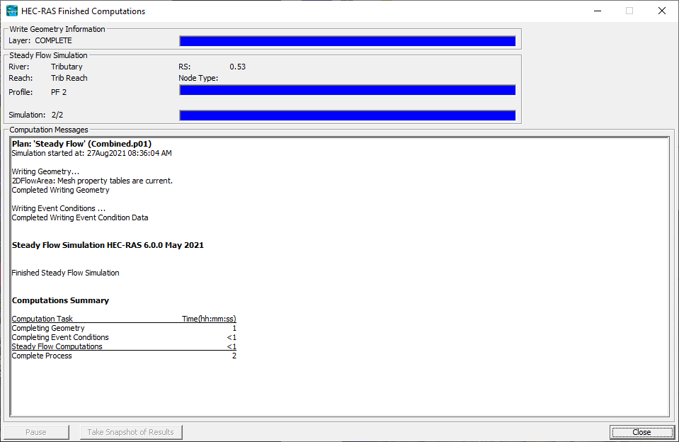
After a completed run, you will be able to examine the model results and refine your model.
1D Model Evaluation and Refinement
Often when developing a model for a river system, the modeler comes the the river with little knowledge of how the system reacts to various flow conditions. While developing the river centerline, flow bath lines, and bank lines you can get a sense for how the river and floodplain will behave. However, the inundation depth, velocity, and boundary visualization provides a "first look" into the soul of the system. Developing the 1D river hydraulics model allows you to quickly gain an enormous amount of insight. Quickly, you will figure out just how little you actually know about the river...and how much you need to modify your initial geometry, before you develop the more complicated unsteady flow model.
Cross Section Improvements
Running the steady flow model with the range of flows is allows you to quickly identify how to improve cross section layout. Using the simulation results, you will see locations where channel banks should be adjusted, locations to add cross sections (or remove), extend cross sections (or shorten), re-align to be perpendicular to flow, or to improve for inundation mapping.
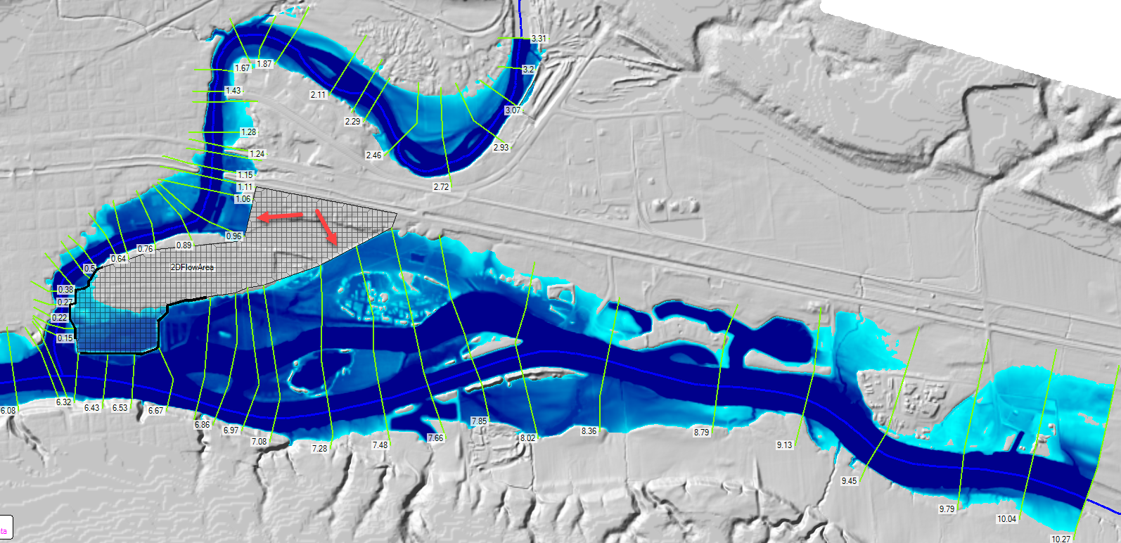
In the below example, there are several cross sections (shown with red arrows) where the floodplain has been limited based on the cross section layout. There may be alternatives to cross section extension, however, for this example it is an appropriate improvement.

For this example, the river channels and floodplain are fairly well defined and reshaping the cross sections was not necessary to improve the model. However, there are still several locations which require improvement. As shown in the image below, there are additional locations (shown with red arrows) where the cross sections should be extended to capture the floodplain. We will improve these designated locations with a 2D Flow Area in a later step.

Inundation Mapping Improvements
There are several other locations where the inundation mapping is not correct. This is especially visible around the levee at the confluence of the rivers. Why are there problems with the inundation? HEC-RAS connects the ends of the cross sections with what are called "edge lines" and the shape of them is created based on the shape of the river and bank lines. The most downstream part of the river we can improve by adding an additional cross section.

Improving the cross section can fix many mapping issues that you may run into. However, with enough modeling you will soon find that no amount of cross section manipulation can give you the mapping results you want the model to accurately reflect the hydraulic results. Take a look at the levee system and inundation mapping inconsistencies. Even with adding the new cross section, the river-side of the levee is still dry. There are still the problems on flooding on the interior side.

To improve the inundation mapping, you have the ability to edit the Edge Lines layer (grouped under the Cross Sections Layer). When you stop editing an edge line feature, RAS will make sure that the edge lines are connected with the end of the cross sections and provide a warning message that the edge lines are going to be modified. Further, the Edge Lines layer will now be saved in the results output during the simulation.


The resulting floodplain mapping is now hydraulically correct, as shown below.

Create 1D Unsteady Flow Data
After creating, examining, and refining the 1D model it is time to move on to an unsteady flow model. Begin by opening the Unsteady Flow Data editor and providing unsteady flow data and boundary conditions.
For this example we have a two river, three reach system. Therefore (at a minimum), we need to specify flow hydrographs at the upstream river stations for each river and specify the downstream boundary condition. We will use the same Normal Depth boundary condition as we used in the steady flow simulation. Use the Flow Hydrograph option for each river. To add a flow data, select the cell corresponding to the river reach and click the Flow Hydrograph button.

Enter the flow hydrograph using the provided table or use a connection to a DSS file. An example hydrograph data entry is shown below.

After entering information, always use the Plot Data button to verify the data entry! An example hydrograph plot is shown below.

Enter the downstream boundary by selecting the corresponding cell and clicking the Normal Depth button. Enter the normal depth slope as shown in the figure below and press OK.

Save the unsteady flow data using a useful name.

You are now ready to create an unsteady flow plan and simulate.
Create 1D Unsteady Flow Plan
Create the initial unsteady flow plan. Most likely there will be some data that you have need to complete, which the interface should report to you, or you model will go unstable. In either case, make sure to make thoughtful decisions for the Simulation Time Window, Computational Time Step, and other Computational Options and Tolerances.
Save the plan with a descriptive name.
Setup the unsteady flow plan with a simulation time window that is short before you try to running a long simulation. Evaluate a time step that will satisfy the courant condition. Time step selection will be based on the cross section spacing and velocities.

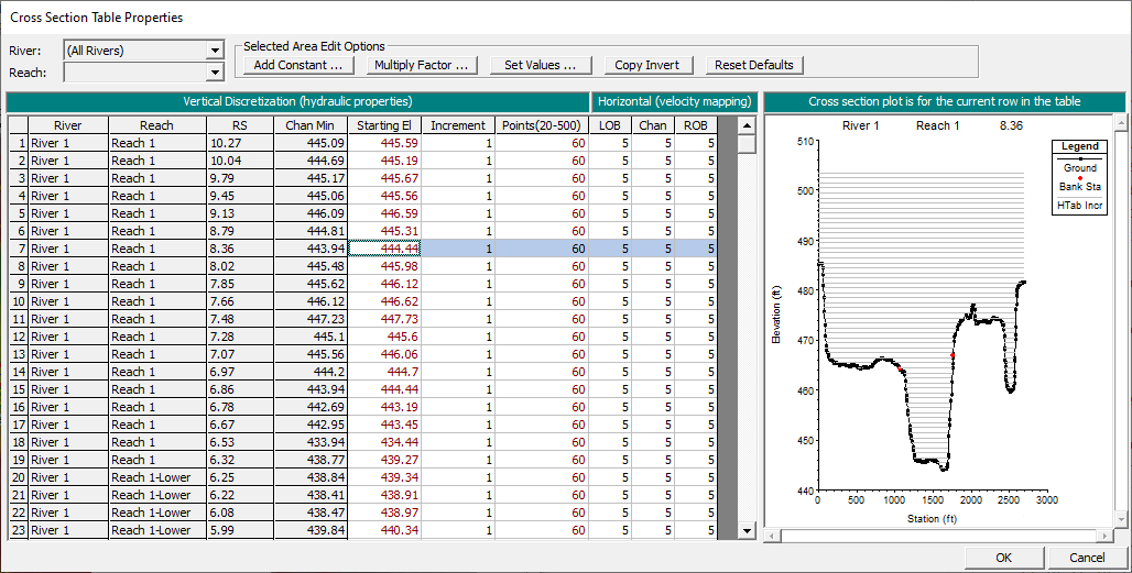
A common error when moving from a steady flow to unsteady flow simulation is to forgot to set up the hydraulic table parameters for cross sections. If the parameters are not set, HEC-RAS will report the missing data when the simulation attempts to begin.

To update the cross section table properties, select the Hydraulic Table Parameters button from the Geometric Data Editor. Copy the invert to the Starting Elevation column and then add a value (the default used by RAS is 0.5ft). Set the number of points to cover the full range of water surface elevations expected to be generated from the range of flows. You can evaluate the stage range by scrolling through each cross section and looking at the vertical slicing in the plot on the right side of the window.
Simulation
After pressing the Computation button, a status dialog (shown below) will provide progress and messaging during the simulation.

If the simulation goes unstable right away, it may likely be due to initial or boundary conditions. A typical example is shown here where the instability is occurring on the tributary reach. You can see this by looking at the computation output and observing that the simulation is going to maximum iterations at the most-downstream cross section for the tributary. This is due to the combination of relatively steep tributary reach coming into the main river which has computed a very low initial water surface (see image below).

The unsteady equations are unable to solve at the junction due to poor geometric data. Bad geometric data, where the geometry is changing more rapidly than it should or is not consistent with the surrounding geometry, is often the source of model stability. For the case of junctions, HEC-RAS has an option to attempt to solve data inconsistencies. The default solution method at a junction is to force the same water surface at all cross sections. Using the method to compute the water surface elevations using an energy balance can help stabilize the model.

Simulation after turning on the "energy balance method" allowed the run to completion.

Simulation results with the water surface elevation computed across the junction look acceptable.

Create 2D Geometry
Once the 1D unsteady flow portion of the model is running stable, only should you consider adding 2D Flow Areas.
2D Flow Areas
For this example, we are adding the a 2D mesh for the area between the river and tributary. The 2D flow area boundary should follow the cross section edge lines. When finished creating the 2D Flow Area, you will be asked to provide a name.

The 2D Flow Area editor will then be invoked. Enter a default cell size and default Manning's n value. For this example, the spatial n values will be used. Generate Computation points for the initial mesh. Consider starting with a large cell size and refine down to a smaller cell size as you become more comfortable with the model.

The initial 2D flow area with computation points is shown in the figure below.

Lateral Structures
The 2D flow area is connected with the 1D portion of the model with lateral structures. Lateral structures should be placed along high ground at the ends of cross sections. Typically, we think of high ground as levees and roadways, but sometimes high ground can be more subtle. Another consideration with lateral structures is that if you need to know how much flow is passing over a certain location, you will need to limit the length of the lateral structure. If you are not concerned with flow accounting, you can create very long lateral structures.
Looking at the 1D unsteady flow model results will determine where to flow will move from the 1D to 2D model. Create the lateral structures in the downstream direction and RAS Mapper will pick up elevations for the weir crest from the Terrain model.


Lateral structure parameters will need to be entered from the Lateral Structure Editor. You will need to set the Tailwater Connection to the 2D Flow Area. You will also need to set the weir coefficient and verify the distance to the upstream cross section.

When you run the simulation, RAS will verify that the elevations of the lateral structure are higher than the minimum elevations of the connected 2D cells. You will receive a warning message if the lateral structure elevation is "below ground", as show below.

You can manually adjust the elevations or use the Clip Weir Profile to 2D Cells button on the Lateral Structure Editor. Before doing that, however, it is a good time to filter that lateral structure elevation points. The elevation profile from the terrain many hundreds (1000 is the default in RAS Mapper), but it is likely that the profile could be adequately defined by much fewer. Fewer points will mean feature computations with the unsteady flow engine because HEC-RAS computes the water surface between each set of points along the weir profile.
The weir profile is filtered using the Filter button on the Lateral Weir Embankment editor, as shown below.

After filtering the data, use the Clip Weir Profile to 2D Cells button on the Lateral Structure Editor (shown below) to ensure the weir profile is higher than the 2D cells.

Combined Model Simulation
After setting up the 2D portion of the model. Then carefully connect the 2D flow area to the 1D geometry. Careful inspection of overflow areas will guide you in using lateral structures to move water between the 1D and 2D domain. However, you do not need to connect the model in every location. Consider adding into the model only one lateral connection at a time.
Time Step Considerations
It is not atypical for your first 1D/2D combined model simulation to go unstable. You can see the initial run begins to iterates to the maximum iterations in the 2D cells. For this example, the 2D cells are much smaller than the distance between cross sections; therefore, we should be using a smaller timestep in for the 2D domain.

A smaller time step is achieved using Time Slices option, located in the 2D Flow Computation Option and Tolerances.

Lateral Structure Parameters
If you continue to have issues with stability (reaching max iterations at cross sections), consider the Weir Flow stability factor.

In our case, after the model became fairly stable, we still had a Volume Accounting that was in error.

Further, consider how the terrain and flow is interacting. Is the high ground along the lateral structure actually working like a levee? Lowering the weir coefficient can be used to dampen the effect of flow leaving the river system. After looking at the flow depths and terrain in detail around lateral structure on the tributary reach, we see flow really isn't controlled like a weir, it is more like overland flow. For the lateral structure in question, change the Overflow Computation Method to the Normal 2D Equation.

Changing the computational method results in fewer iterations, a model that runs faster, and a smaller volume accounting error.

To further improve the volume accounting, we could decrease the timestep which would result in less flow being moved from the 1D domain to the 2D mesh during a single timestep. However, smaller timesteps will result in longer model run times.
Combined Model Evaluation and Refinement
After achieving model stability with the initial combined model, we can visualize results and get a handle on the system performance and resulting inundation. In the below image, we can see area where we should have included lateral structures to connect the floodplain to the river at the upstream end of the 2D flow area.
Continue to add lateral structures where appropriate to model the movement of water in the river system. In the image below, you can see we have added two more lateral structures to allow water to move into the 2D flow area. Be sure to complete all of data for each lateral structure. This includes selecting the headwater location, tailwater location, filtering the elevation profile, selecting a weir equation coefficient, selecting the modeling method, and verifying the headwater distance to the upstream cross section. You will also need to verify that the weir profile is higher than minimum elevation of the neighboring cells.

Evaluate the resultant floodplain for areas of improvement. This can be done using the various output plots in HEC-RAS and map output in RAS Mapper. Take a look at the inundation extent. Animate through the simulation profiles and look for discrepancies in how the water is moving through the system. Evaluating the courant number and velocities will provide insight to the current solution.
Courant Number
Plotting the courant number will help provide further understanding on the interaction of the selected timestep with the cross section spacing and the time slicing for the 2D flow area. Striving for a courant number near 1.0 is a noble effort, but can rarely be achieved for the entire model. If you identify particularly sensitive areas to the selected timestep, reduce and rerun.

Velocities
The velocity map is ideal map for gaining insight to the river and floodplain. Create a velocity map and animate through the profiles. Pay special attention to high velocity locations or where velocities change rapidly.

Not that if you plot the Max velocity, you will not get the a map that looks like any of the profiles that you animated through. This is because the maximum velocity is output separately from the data export at the "Mapping Output Interval" specified on the Unsteady Flow Data Editor. Investigate the max velocities to identify if it is the result of model instability or if the output interval did not catch the higher velocity. For the example shown below, the max velocity is reporting very high velocities near structures that are overtopped (that are not shown in the animation of the output). This is most likely due due to the diffusion wave solver struggling to solve for a stable solution just as the structure is overtopped.

Make a run with the model, setting the mapping output equal to the time step. This will plot all of the computed results and allow you to see values that may have been skipped over. Zooming into the high velocity region, you can see the model is going unstable. Below is a depth plot for one of the cells showing how the depth is flipping between wet and dry. This indicates that the computed water surface elevation is very sensitive to the 1D/2D connection. This may be due to the weir coefficient or the location of the weir resulting in a poor elevation profile. Or maybe the timestep is just too big. Or a combination of factors.
In the below plot of the water surface time series, you can see the water surface oscillating - the 2D cell is wetting and drying every other timestep.

Plotting the time series of depths for the cell, you can see the large changes each timestep.

This demonstrates the importance of placing lateral structures on high ground and have the correct weir elevation profile. If we had survey information we could replace the weir profile. In order to fix this issue, we will need to move the lateral structure to high ground and adjust the edge of the 2D flow area.
Moving the lateral structure to high ground improved the solution and kept the water surface for moving out into the 2D area prematurely, iterating, and poor mapping. No longer due we have max velocity issue in this area, as shown in the max velocity mapping below.

Because lateral structures control flow into 2D flow areas and cell faces control how water moves within the 2D flow area, you must take precaution to ensure these controls are on high ground. Poor placement of cell faces and structures may not result in final water surface elevations that differ from the "perfect" solution, however, than can cause model instabilities that result in longer run times, volume accounting errors, local mapping issues, and other local anomalies. Take care to address each issue to improve model fidelity.
You may find yourself in the situation (shown below) where the Max velocity doesn't match any of the values contained in the output, despite setting the Mapping Output Interval equal to the Computation Time Step. This can happen if you have time slicing turned on. The max value could occur in the 2D cell during a time slice and not be reported at the output interval.
Model Sensitivity and Comparison
After reviewing initial model results and refining the geometry for river hydraulics model, you should spend more time trying to identify parameters in the model that are particularly sensitive. Hopefully, you have already been doing this initial investigation as you found model instabilities or data inconsistencies with previous simulations. There are many model data and parameters that may or may not impact the simulation results that are worth discussion. Saving an existing Plan to a new name and rerunning the model allows for an easy way to look at the affect of simulation parameters.
Parameters
One of the most important parameters that should be evaluated is the effect of the simulation time step on the model. Additional parameters that can and should be considered can be found on the Computation Options and Tolerances window. Some of the more important parameters are discussed below.
Time Step
You should always evaluate the affect of the computation time step on the hydraulic results. If reducing the time step resulted in significant changes to the water surface elevations or velocities, then the smaller time step should be used for future simulations. Various time steps should be evaluated and their effects on model stability, accuracy, and computational run time.
If you would like to have HEC-RAS figure out a time step to use base on the courant criteria, you can use the Advanced Time Step Control available on the Computation Options and Tolerances window.
Time Slices
The computation time step effects the base unsteady flow computation engine. For a combined 1D/2D model, if you require a smaller time step for the 2D Flow Areas, you must use the Time Slicing option. The optimal value can be identified through trial and error balancing model stability, accuracy, and computational run time.
Equations Set
2D model runs have the option to run either the using the Full Shallow Water Equations (SWE) or with the Diffusion Wave (DW) approximation of the momentum equation. The diffusion wave approximation is appropriate in where the dominant forces on flow are mainly gravitation and friction forces. Where local convective acceleration is important, the full shallow water equations will be more appropriate.
Once a model is up and running, you need to compare runs with the SWE to the DW. If you model shows significant difference, you should be using the SWE for all future model runs.
- Diffusion Wave - DW is more computationally stable and good for getting a 2D model up and running to get a rough estimate for inundation extents and depths. For complicated problems, DW is simply a first step before applying SWE. Some key points are listed below.
- Very stable
- Not good for rapid rising/falling hydrographs (temporal acceleration)
- Not good for sharp contractions and expansions (accelerations)
- Not good for sharp bends for modeling super-elevation
- Not good for tidal boundaries (no wave propagation)
- Can't model hydraulic jumps
- Full Shallow Water Equation - SWE is important for modeling rapid changes to flow due to acceleration whether that be do changes in hydrograph or geometry that results in rapidly varied flow. Some key points are listed below.
- Less stable than DW requiring a smaller time step and longer computation times
- Needed for rapid rising/falling hydrographs (temporal acceleration) like dam and levee breaches
- Needed for sharp contractions and expansions (accelerations) like at hydraulic structures like a bridge opening
- Needed for sharp bends for modeling super-elevation
- Needed for tidal boundaries (no wave propagation)
- Needed for modeling hydraulic jumps
Theta Implicit Weighting Factor
Theta is the implicit weighting factor used by HEC-RAS for solving the unsteady flow equations. The default value of 1.0 is the most stable and uses information on from the current time step weight the pressure gradient term in the momentum equation to solve the unsteady flow solution. Using a value smaller than 1.0 will result in the using the information from the previous time step with information from the current time step during the solution. HEC-RAS allows for a value of 0.6 to be used for the most accurate solution (at the cost of stability).
Stability Factors
Stability factors have been added in HEC-RAS to to keep flow from rapidly changing during the simulation. Experience has shown that dampening flow over lateral structures can greatly improve model stability. One the model is stable, these factors can be decrease back to a more accurate solution.
- Lateral Structure Flow Stability Factor - This factor ends up reducing the amount of flow change between time step at a structure. A value of 1.0 is the default and more accurate. A value of 3.0 will end up reducing flow and increase model stability.
- Weir Flow Submergence Decay Exponent - This factor is used to reduce the amount of flow over a weir that is submerged. Submergence occurs when the tailwater is high enough to slow down flow. Rather than waiting until the weir is highly submerged, weir flow can be reduced sooner resulting in smaller changes in flow and more model stability. The default value of 1.0 uses the default flow reduction. A value of 3.0 reduces under less submergence and is more stable.
Turbulence Modeling
Turbulence modeling can be important in 2D unsteady flow modeling where slow water attempts to slow down faster water and fast water attempts to speed up slower water - the action that produces eddies. Turbulence modeling is only available when using the SWE because the DW approximation ignores all terms except the pressure gradient and bottom friction terms. Turbulence modeling requires the selection of a longitudinal mixing coefficient, transverse mixing coefficient, and Smagorinsky coefficient.
Model Comparison
To understand the model's sensitivity to each of the model parameters previously discussed, you will need to establish a base plan and then compare those results with various alternatives. There are many tools available for results comparison.
Profile Plot
An example profile plot from HEC-RAS is shown below for a single river reach with the max profile for two plans.

XS Plot
An example cross section plot from HEC-RAS is shown below with the max profile for two plans.

Hydrograph Plot
A hydrograph plot from RAS Mapper is shown with a water surface elevation time series plot for two simulations. Output is available from the map for whichever mapping results are visible.

Profile Lines
An example profile plot from HEC-RAS is shown below for a river reach with the max profile for two plans. Output is available from the map for whichever mapping results are visible.

Watch List
The Layer Values Watch List is created by right-clicking on any layer and choosing the Add Watch to Layer Values menu item. As you move the mouse across the map display, the cursor will report the map value next it's label (ID) as well as reporting the value in the Layer Values dialog. This is a valuable tool for a comparison of computed map results. Example output is shown below.

