Download PDF
Download page Bridge Analysis.
Bridge Analysis
Data Files
You will be working with a section of Beaver Creek located near Kentwood, Louisiana. The data for this tutorial is provided in the zip file.

Objective
This workshop will help students learn how to use HEC-RAS to perform water surface profile computations through a bridge. Students will review and understand pertinent bridge output for the different modeling approaches and adjust the geometry to improve the bridge solution.
This workshop is a continuation from the previous Bridge Development workshop that guided student though adding a bridge to an existing geometry.
Background
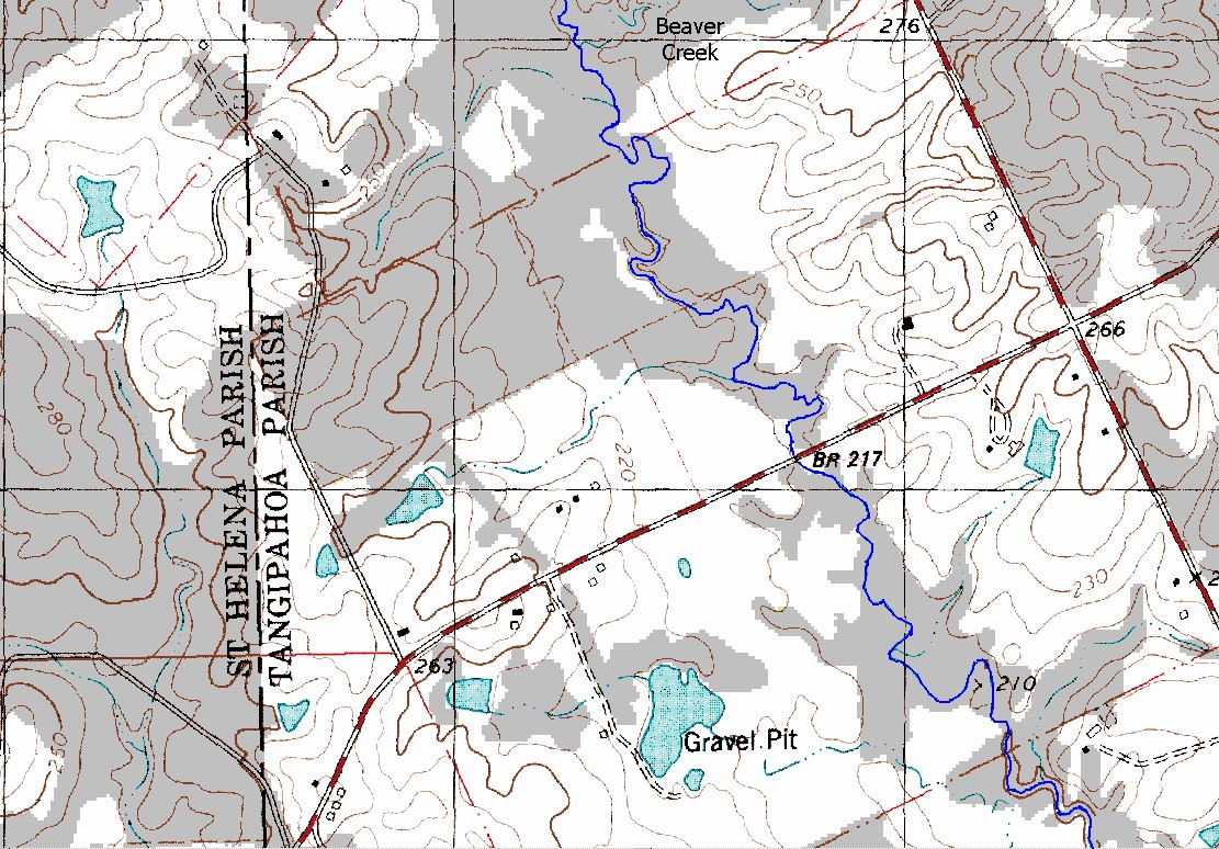
The stream for this example is a section of Beaver Creek located near Kentwood, Louisiana. The bridge crossing is located along State Highway 1049, near the middle of the river reach. The field data for this example was obtained from the USGS study “Backwater at Bridges and Densely Wooded Flood Plains, Beaver Creek Near Kentwood, Louisiana” by George J. Arcement, B.E. Colson, and C.O. Ming.

Compute Steady Flow Plans
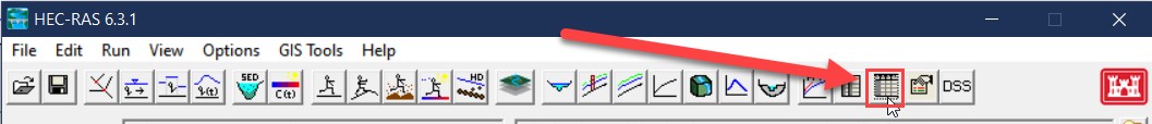
- Start HEC-RAS
- Open the “BridgeAnalysis” workshop in the Bridge Analysis Workshop folder.
- Note if you are confident in your work, use your completed Bridge Development workshop as a starting point.
- Compute each of the plans:
- “Bvr Crk” : Existing geometry without a bridge
- “Bvr Crk Br.–Energy”: Geometry w/ bridge using Energy for High Flow
- “Bvr Crk Br.-PW”: Geometry w/ bridge using Pressure Weir for High Flow
Review Initial Results
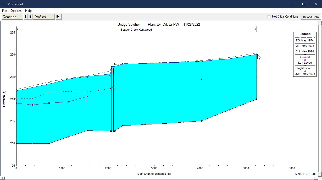
- Compare the initial results of the three plans using the Cross-Section Plots and Profile Plots. Answer the questions below.
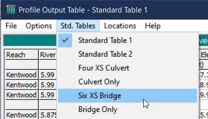
The energy method resulted in the highest elevations upstream of the bridge. The Six XS Bridge Table was used to compare WSELs between plans at each cross-section.
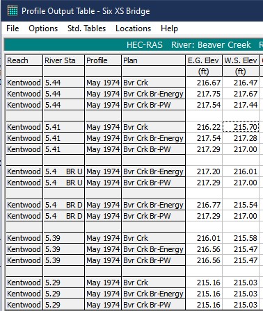
In comparing the profiles for the with bridge and without bridge plans, backwater from the bridge impacted WSELs all the way to the upstream cross-section of the reach (approximately 2900 ft upstream).

The pressure / weir method is more appropriate for the high flow event. That is because it is being overtopped such that the road embankment is behaving like a long weir. Additionally, the bridge inlet is submerged so flow through the opening the is behaving like sluice flow. If this bridge was grossly overtopped and highly submerged, we may consider using the energy method for high flow instead.
After calibrating the submerged inlet coefficient, the pressure / weir method compared well to the observed WSELs. However, the energy results were not far off from observed data either.
Compare Computed Results with Observed Data
Lucky you, there are observed data for the 14000 cfs event that occurred 22 May 1974. The USGS observed high water marks are provided below.
Cross Section River Station | Observed WSE (ft) |
5.99 | 220.0 |
5.76 | 218.4 |
5.61 | 218.1 |
5.44 | 217.8 |
5.41 | 217.8* |
Bridge 5.4 | |
5.39 | 215.2* |
5.29 | 214.9 |
5.13 | 213.6 |
5.0 | 211.8 |
*The observed high water mark at this location is questionable.
- Enter the Observed High Water marks for each cross-section in the Steady Flow Data Editor
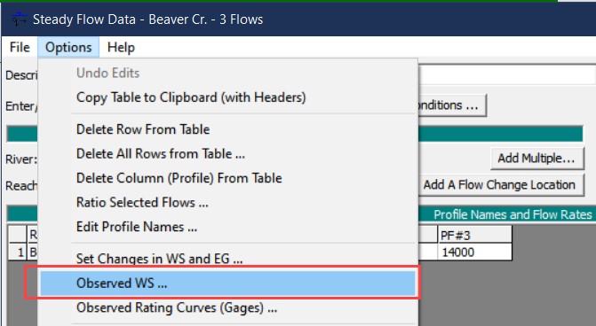
- Compute and compare results against observed
Adjust the Submerged Inlet Coefficient for Pressure Weir
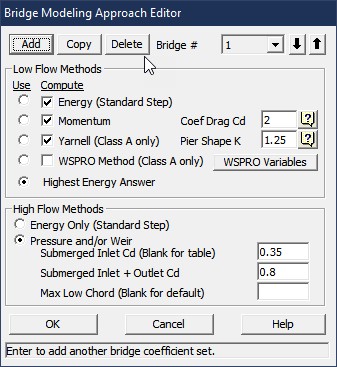
- Calibrate the Submerged Inlet Coefficient (Cd) for the bridge in the pressure weir Geometry to better match the observed high water marks for the May 1974 profile.
- A reasonable range for Cd values from the HEC-RAS Hydraulic Reference Manual is 0.27 – 0.5
Adjust Ineffective Flow Areas for the Pressure Weir
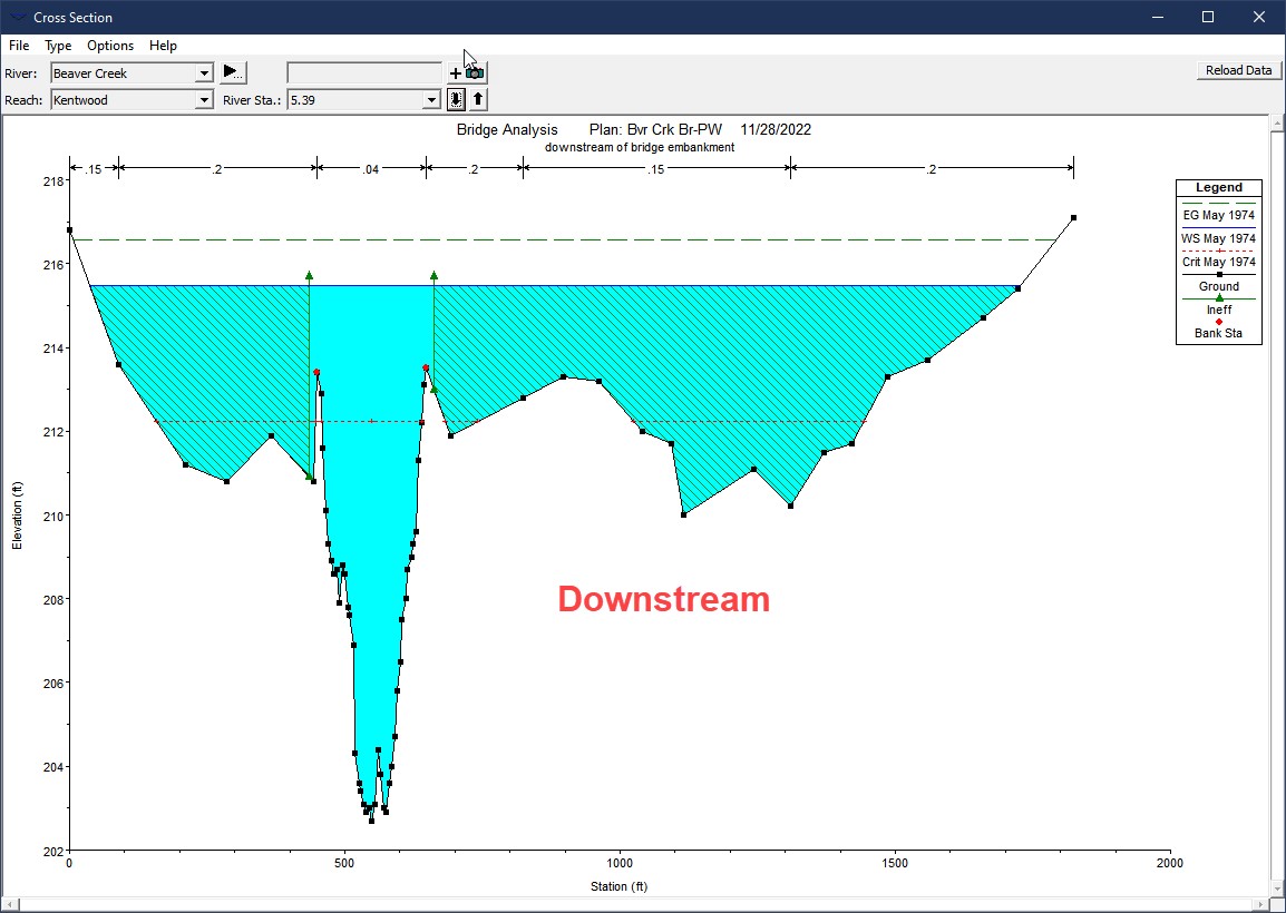
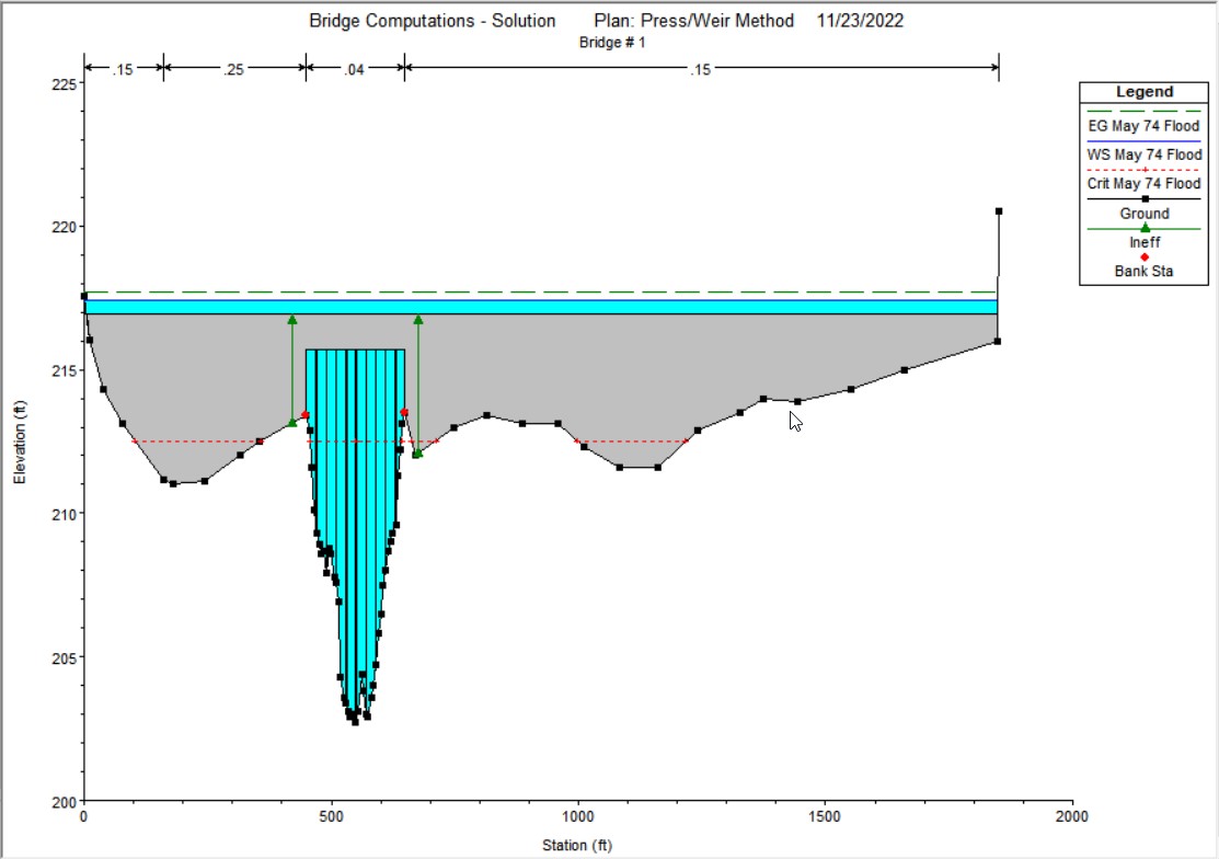
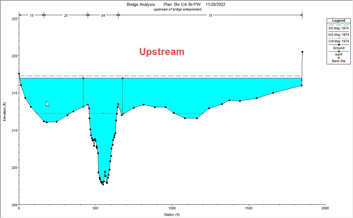
- Looking at the bridge cross section plot for the May 1974 profile, adjust the trigger elevations of the ineffective flow areas for the pressure weir bridge Geometry.
- When using pressure weir, the goal is for the ineffective areas to turn off as the energy grade exceeds the roadway on either side (i.e. when we begin to compute weir flow over the roadway).
The downstream ineffective flow areas were not turning off in sync with the upstream ineffective flow areas. That said the downstream trigger elevations had to be lowered.
No adjustment was needed for the upstream trigger elevations. That is because for the only profile in which the energy grade exceeded the bridge deck (and weir flow occurs), the ineffective flow areas were already triggered off by the water surface elevation. So, setting the ineffective flow areas at the top of the bridge deck for this profile was fine.
Adjust Manning’s n to Balance Bridge Flow
When using the pressure weir method, the flow in the overbanks of the upstream and downstream cross-sections, should be reasonably close to the weir flow over the bridge roadway. In order to balance the flow distribution in the cross sections, you will adjust Manning’s n for the upstream and downstream cross-sections.
- Create a new Geometry from the pressure weir geometry and call it “Bvr Crk-PW-Balance”. Create a new corresponding Plan.
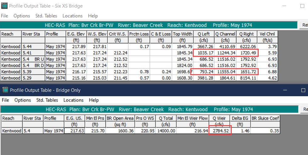
- For the pressure weir Plan, open the Six XS Bridge Table, and the Bridge Only Table.
- Compare the total overbank flow at the upstream cross-section (5.41) to the weir flow for the bridge.
- Adjust the overbank Manning’s n value in the upstream cross-section in an attempt to match the brdige weir flow to the total overbank flow.
- Note you the total weir flow includes the weir flow over the center of the bridge as well.
- Similarly, adjust the downstream cross-section Manning’s n to match the weir flow.
The flow in the overbanks for the cross-sections upstream and downstream of the bridge exceeded the weir flow for the bridge. In order to balance the weir flow with the overbank flow, the Manning’s n values were increased for the cross-section overbanks until the flows were more balanced. The Six Bridge XS Table and the Bridge Only Table were used to compare weir to overbank flow. For this dataset the water surface profiles were not noticeably impacted by adjusting the Manning’s n to distribute flow appropriately around the bridge.