Download PDF
Download page Calibration of a Steady Flow Hydraulics Model Workshop Solution.
Calibration of a Steady Flow Hydraulics Model Workshop Solution
Data Files
You will be working with a section of Trinity River downstream of Lewiston Lake near Weaverville, CA. The data for this tutorial is provided in the zip file.

Introduction
This workshop will help students learn how to use HEC-RAS to calibrate a steady flow hydraulics model. Students will learn how to adjust parameters to replicate observed water surface elevations for three different observed events. While this data is from an actual study, the model and results of this workshop do not represent current or future conditions of the river system. This data is provided as a teaching example for purposes of instruction only.
Background
In 1958, a plan was developed to increase water supplies and generate power for California’s Central Valley in part by transferring water from the Trinity River into the Sacramento River. Completed in 1964 for these socially and economically important purposes, the Trinity River Division (TRD) of the Central Valley Project began a decades-long era wherein up to 75-90% of the inflow to Trinity Lake was exported from the river each year. Figure 1 shows the Trinity River below Lewiston Lake near Weaverville, CA. Lewiston Lake is a flow re-regulation lake that is just below Trinity Dam (Trinity Lake).
As you would expect, the natural flows in the Trinity river have changed dramatically since 1964. While sediment supply was being cut off from upstream, more importantly, natural annual flood flows were being cut off from the Trinity river. Prior to the TRD, stream flows varied greatly between and within each year. In a given year, flows could range from as low as 100 cubic feet per second (cfs) during the summer up to over 100,000 cfs during rare rain-on-snow floods. After the TRD was complete, flows were held between 150 cfs and 300 cfs year-round except for occasional storm-response reservoir releases, the largest of which was 14,500 cfs in 1974.
There are many downstream tributaries that come into the Trinity river below Lewiston Dam. Because of the dramatic decrease in flow rates, finer sediments have deposited and filled in the gravel beds that use to support spawning grounds for Chinook salmon and Steelhead. These finer sediments have also allowed tremendous riparian vegetation to take hold on the banks of the main channel, as can been seen in the photos in Figure 2 and Figure 3.
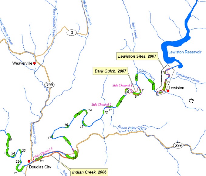
Figure 1. Trinity River below Lewiston Lake near Weaverville CA.
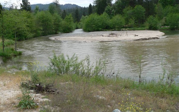
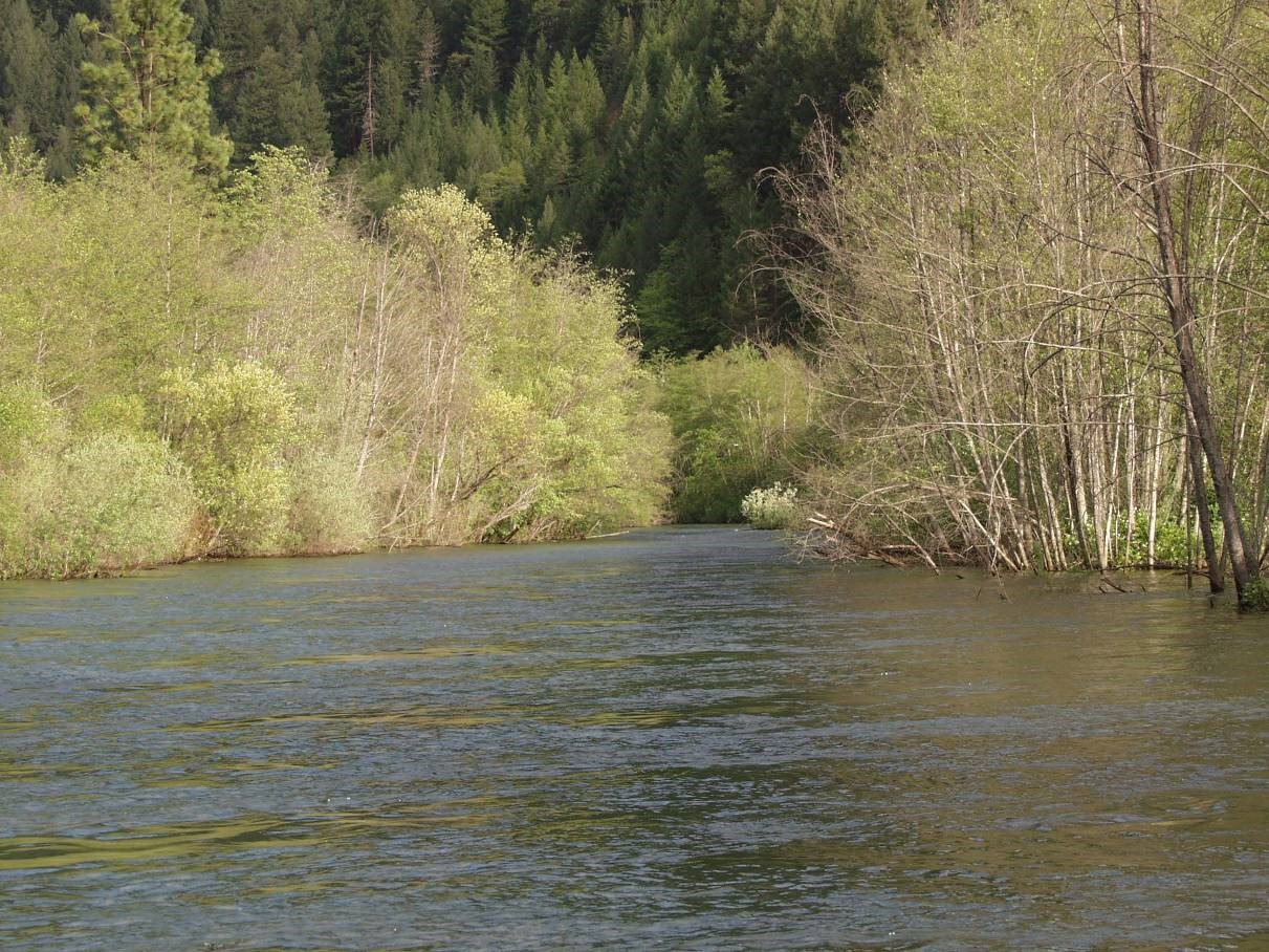
Figure 2. Typical Stream photos of the Trinity Below Lewiston Dam.
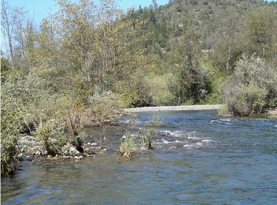
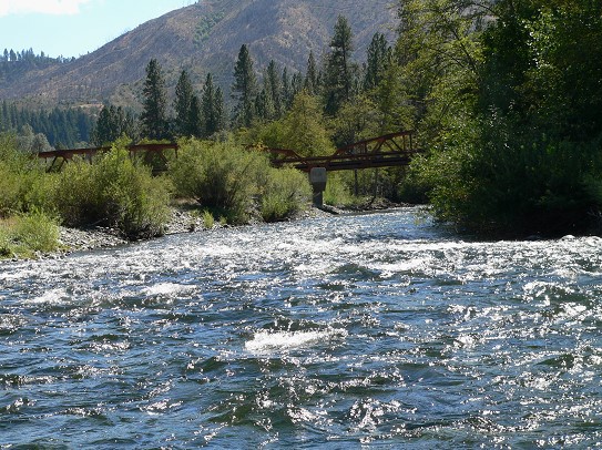
Figure 3. Additional photos of the Trinity River Below Lewiston Dam.
Problem Description
A project file (CalibrationWorkshop.prj) with the title “Calibration Workshop – Trinity River CA” is available for download at the top of this screen. This file contains all the data for this workshop. This model is a short reach of the Trinity River (about 5 miles) below Lewiston Dam, in the area from just above the Indian Creek tributary down to the confluence with Weaver Creek, near Douglas City. All of the Geometry and flow data are already in the project file.
The flow data file contains three events: 450 cfs (a typical summer low flow); 4500 cfs and 7000 cfs, both of which were controlled releases from Lewiston Dam. Observed high water marks were surveyed for all three events, and have already been entered into the flow data editor.
This model was originally calibrated to all three of these events. For the purpose of this workshop, all of the main channel Manning’s n values have been set to 0.02 (which is lower than the true final calibrated values). Some hydraulic information about the main channel is as follows:
- Average Stream Bed Slope = 0.0023 ft/ft
- Typical Hydraulic Radius values for the main channel at bank full stage range from approximately 4.0 to 6.0 feet.
- D84 of the bed material in this region has been measured around 80 mm (0.262 ft)
- Main channel banks contain thick stands of trees and vegetations as shown in the pictures above.
Tasks
1. Make initial estimates of the main channel Manning’s n values using the Limerinos and Jarret equations:
Calculate a Manning’s n value for the main channel from both equations but select a single value to start with as your initial estimate that you put into the HEC-RAS model.
Limerinos Equation:
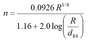
Where: R = Main Channel Hydraulic Radius in feet
d84 = Material size of which 84% of the bed is finer (feet)
n = 0.033 for R = 4.0 ft; and n = 0.032 for R = 6.0 ft.
Jarrett’s Equation:
n = 0.39 S0.38 R-.16
Where: S = Average Bed Slope (ft/ft)
R = Main Channel Hydraulic Radius (feet)
n = 0.031 for R = 4.0 ft; and n = 0.029 for R=6.0 ft.
2. Adjust the main channel Manning’s n Values based on your calculations from Task 1, run the model and review the results, then answer some questions.

Figure 4. Manning’s n value Editor Table.
The easiest way to use the Manning’s n value table to change the main channel n values is to first select to view “Main Channel Only” from the drop down box at the top of the editor. Also, once any changes are made in this editor, you must press the “OK” button to close the editor and have the changes accepted before running the model.
Run the model with your initial set of main channel Manning’s n values. Then answer the following questions:
Based on the calculations from Task 1, it was decided to use a value of n = 0.031 for the initial estimate of the main channel Manning’s n values in the model.
In general the computed results are lower than the observed values for the 4500 and 7000 cfs profiles. In some places the computed values were more than 1.0 feet lower than the observed. There was one portion of the model where the n = 0.031 value seems to be fine, which is in the cross section range from 93.7 to 95.03. Both downstream and upstream from this region, the computed values are lower than the observed for the two higher profiles. Differences are the greatest for the upstream half of the model.
The results of the low flow profile are very mixed. In some places they are good, in some places the computed values are high, and in some places the computed values are low.
A profile plot of the results for the upper reach, profile three (7000 cfs) is shown in the figure below. This is the area of greatest discrepancy between computed and observed values.
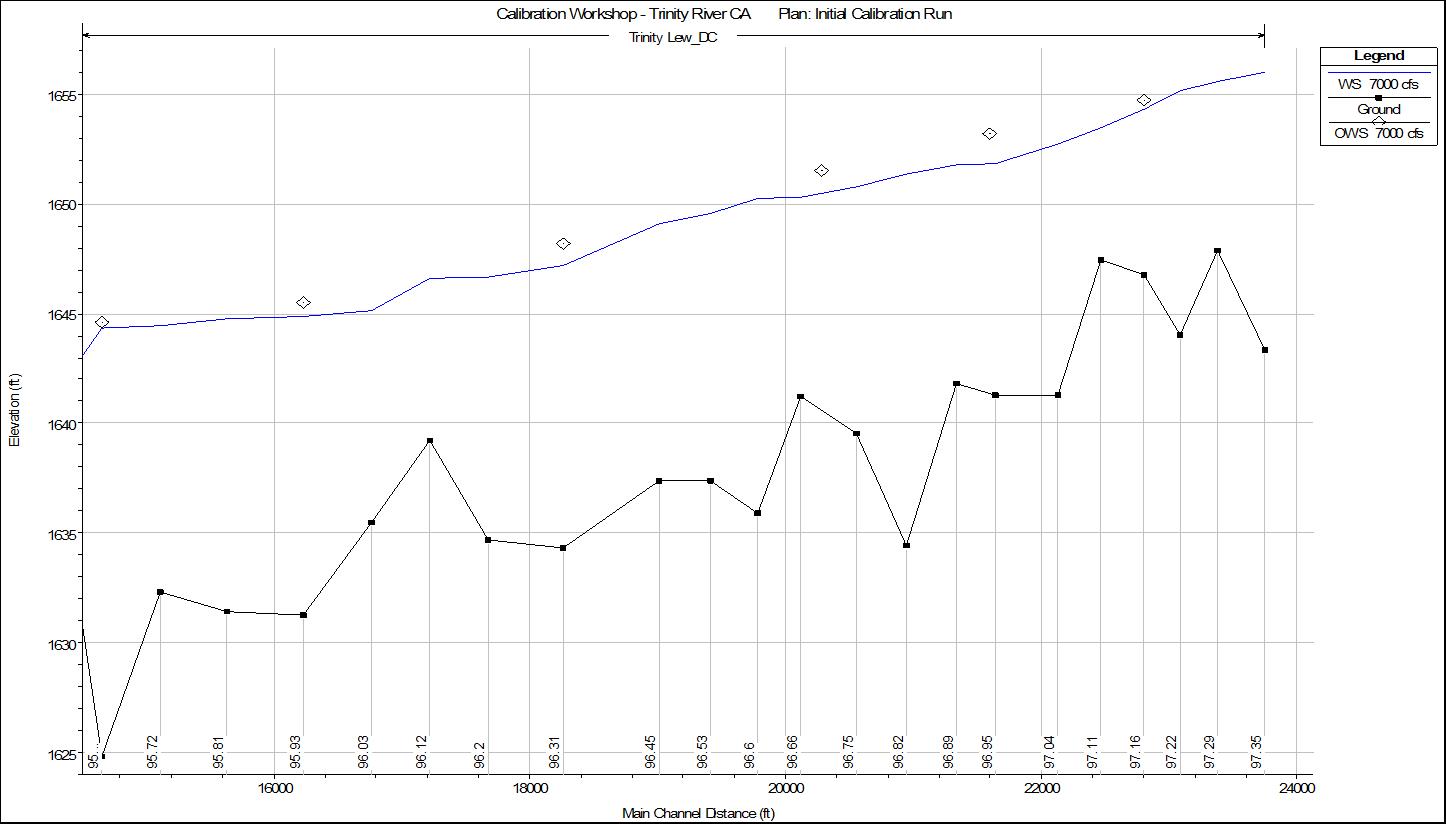
Figure: Computed vs. Observed data for 7000 cfs profile, at upper half of the model.
In general the Manning’s n values needed to be increased at the bottom end of the model as well as the upper half of the model. Based on the pictures provided and the information about the dramatic reduction in flow regime, as well as the knowledge that finer sediments are now settling out in the channel banks and point bars, a tremendous amount of vegetation/trees have taken hold on the channel banks and what previously were gravel point bars. This vegetation will slow down the flow, cause more turbulence, and in effect require a higher Manning’s n value to calibrate the model. Additionally, the upper half of the model goes around a very tight bend, which will also increase flow turbulence and require higher n values to match the higher stages through the bend area.
3. Calibrate the main channel n values to match the observed data.
Adjust the main channel Manning’s n values to better match the observed data. Concentrate mostly on trying to match the 4500 and 7000 cfs profiles. Start downstream and work your way upstream. Remember to change Manning’s n values over a reasonable range of cross sections, not just one cross section at a time.
After you think you have the model calibrated reasonably, answer the following questions:
The range of Manning’s n values for the final calibrated model went from a low of n = 0.032 to a high of n=0.04.
Yes. Values were slightly increased to 0.035 in the lower portion of the model to getter a better fit with the upper two profiles, as well as the low flow profile. Values were adjusted from 0.032 to 0.034 in several portions of the next section of the model (cross sections 93.57 to 95.17). This allowed for a better calibration of all three profiles. A profile plot of this region is shown in Figure A below.
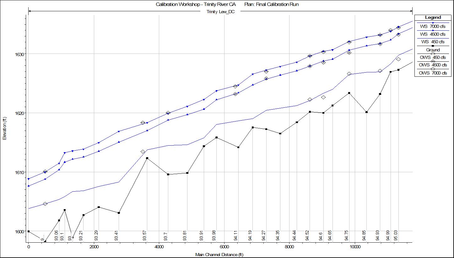
Figure A. Computed vs. Observed data for all three profiles in the lower portion of the model.
Manning’s n values had to be gradually increased from a value of n = 0.035 at cross section 95.3, up to n = 0.04 at cross section 95.93. This produced good results for the upper two profiles, but the lower profile was still below the observed values. A profile plot of the results for this region is shown in Figure B.
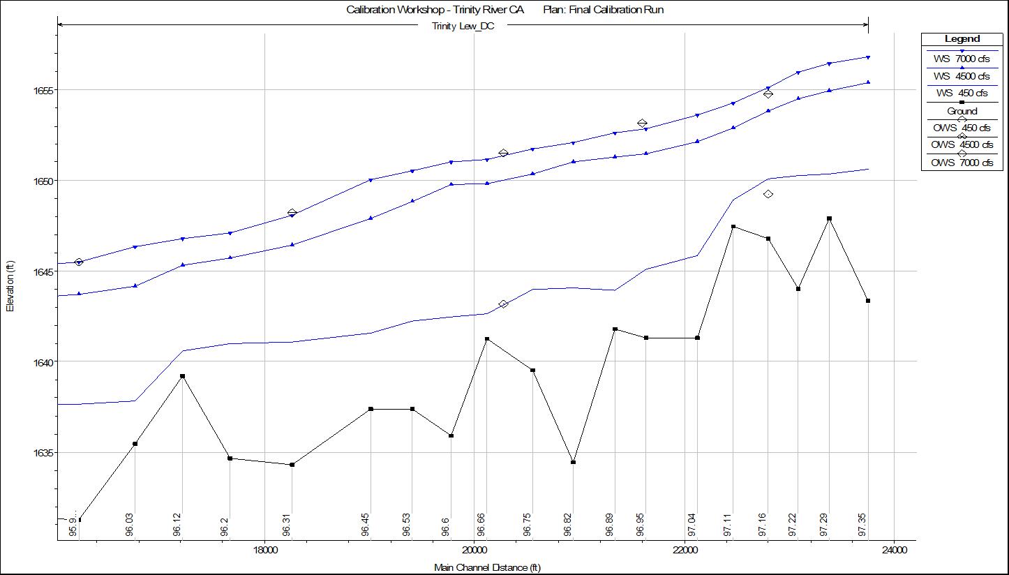
Figure B. Computed vs. Observed data in the middle section of the model.
Manning’s n values were left at 0.04 for the upper portion of the model, cross sections 95.93 to 97.35. This produced good results for the two higher profiles, but mixed results for the lowest profile. A profile plot for the results in this region is shown in Figure C.
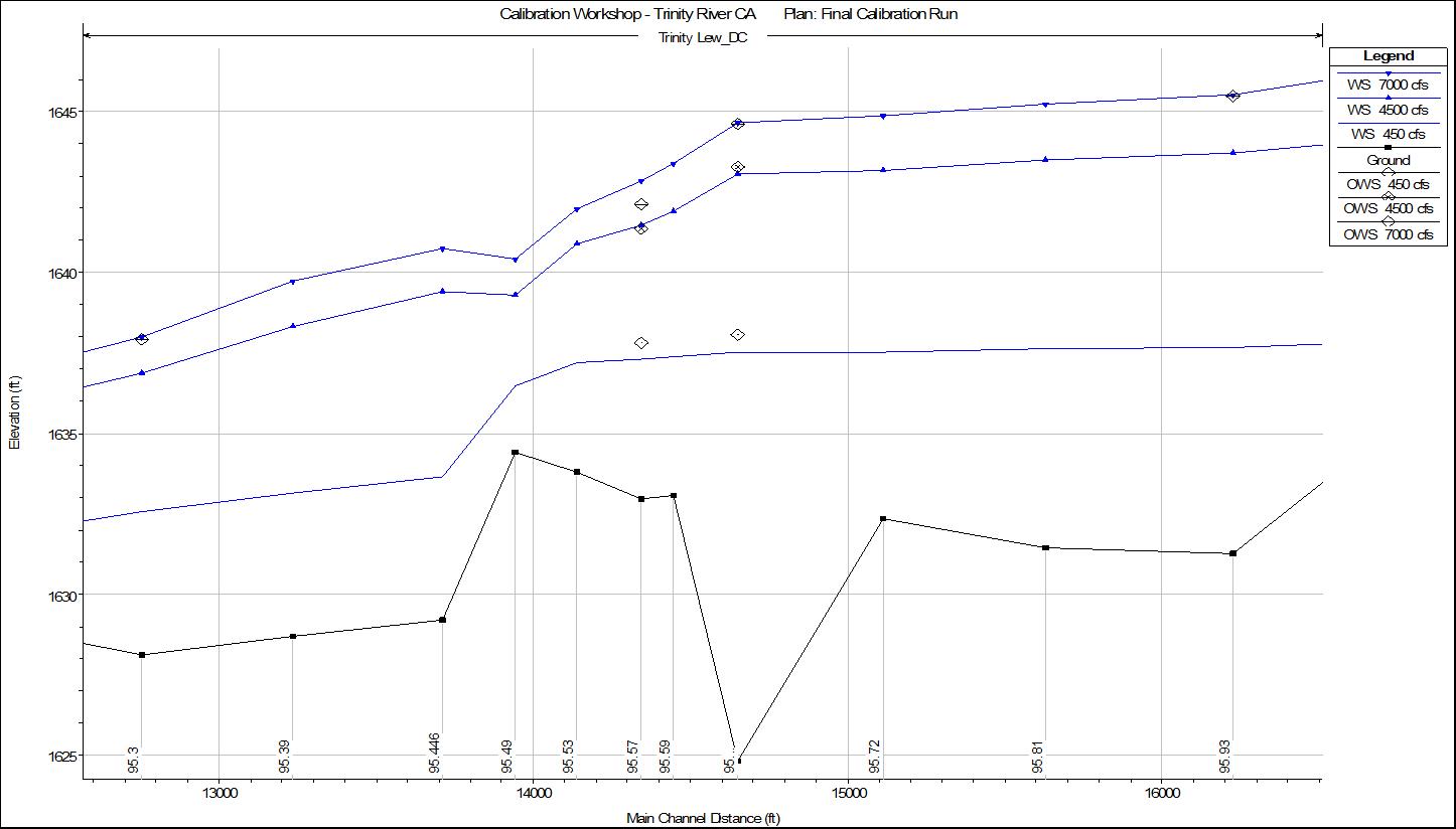
Figure C. Computed vs. Observed data for the upper half of the model.
Yes. The very middle portion of the model (shown in Figure B in the answer above), there is a break in slope both in the bed profile, as well as the computed water surface profiles. In this region the computed values were very good for the 7000 cfs profile, slightly low for the 4500 cfs profile, and very low for the 450 cfs profile. Using a variable n value option here could have improved the model results. The flow versus roughness factors option could have been used in this region to increase the roughness for the lowest flow, and then gradually go back to a factor of 1.0 (no change) as the flow increased towards the 7000 cfs profile.