Download PDF
Download page Culvert Analysis.
Culvert Analysis
Data Files
You will be working with a section of Napa Creek located near Napa, CA. The data for this tutorial is provided in the zip file.

Introduction
This workshop will demonstrate the application of the HEC-RAS culvert capability. A proposed highway crossing of Napa Creek, with twin box culverts, will be analyzed. Figure 1 is a plan view of the study area, from a USGS 7.5 minute quadrangle. The new highway is shown running north-south and the Creek generally runs from west to east toward Napa River. Water surface profiles have been computed for the creek, starting at the Napa River. A local control (critical depth) was found at river station 3650; therefore, this analysis will start at that location.
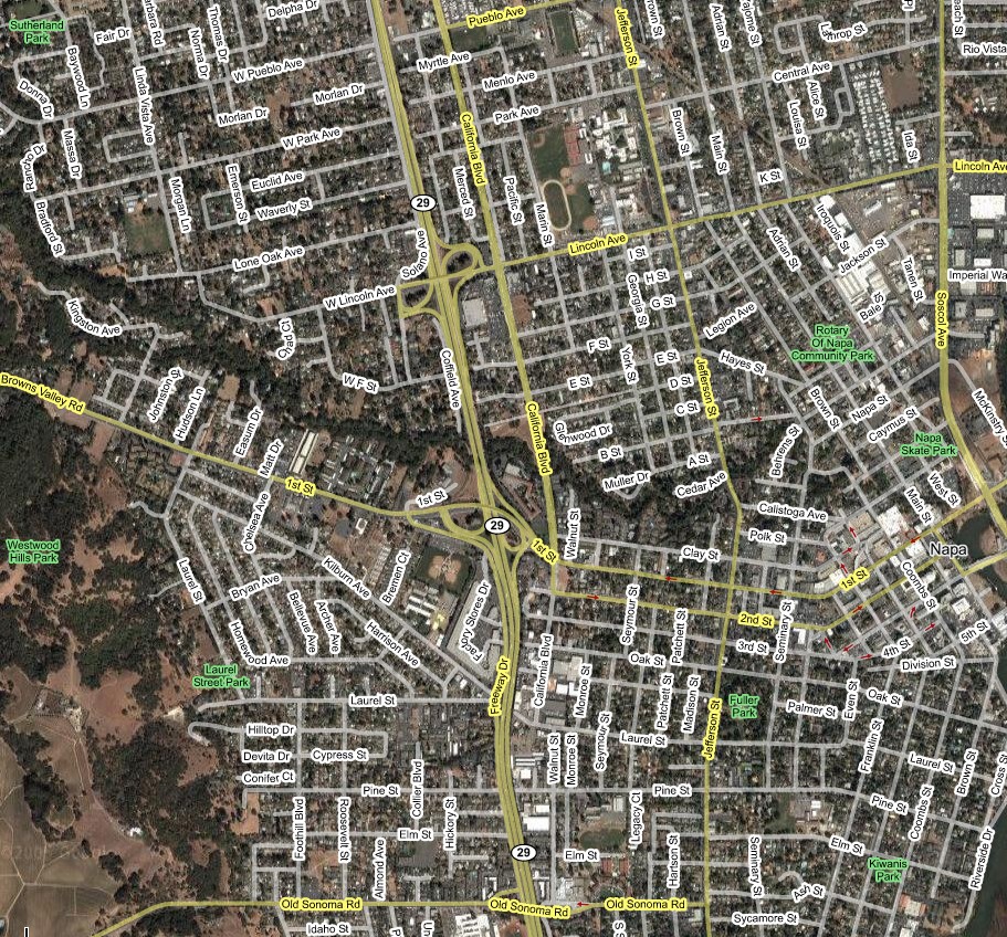
Figure 1 Napa Creek at highway crossing
Problem
The Napa Creek project (filename = WRK3.prj) is the existing conditions data file for the upper Napa Creek, starting at river station 3650. The flow file is Napa Creek - Flood Flows, which includes a recent flood (2,500 cfs), a one-percent chance flow (4,000 cfs) and a maximum flood of 6,500 cfs. All subcritical profiles start at critical depth at river station 3650. The Napa Creek - existing conditions Plan represents the base condition, without the highway crossing.
Part 1
The proposal is to carry the highway crossing over two concrete box culverts. The size and locations are as follows:
- Two 18' wide x 12' high concrete box culverts
- 80' long, centered between river stations 4042 and 4142, see figures below.
- 90 degree head wall, with inlet edges beveled ¾ inch on three sides
- upstream invert = 17.0'
- downstream invert = 16.7'
- Centerline station = 65' and 85'
Select appropriate coefficients based on the tables in Chapter 6, Hydraulics Reference manual. The top-of-road profile is shown, based on cross-sectional stationing:
Station: | 0 | 50 | 100 | 160 |
Elevation: | 36.5 | 34.5 | 34.5 | 37.0 |
The top of the road is 60 feet wide, and the upstream edge of the road profile is 20 feet from the cross section just upstream of the road embankment.
The design requirements state that the one-percent flow profile (4,000 cfs) should not increase more than one foot above base conditions and that the maximum flood (6,500 cfs) should not overtop the roadway.
Part 1 Tasks
- Assemble the necessary added data and run the model with culverts. Don’t forget to set the effective-area option on the adjacent cross sections. Save the geometry file under a new name.
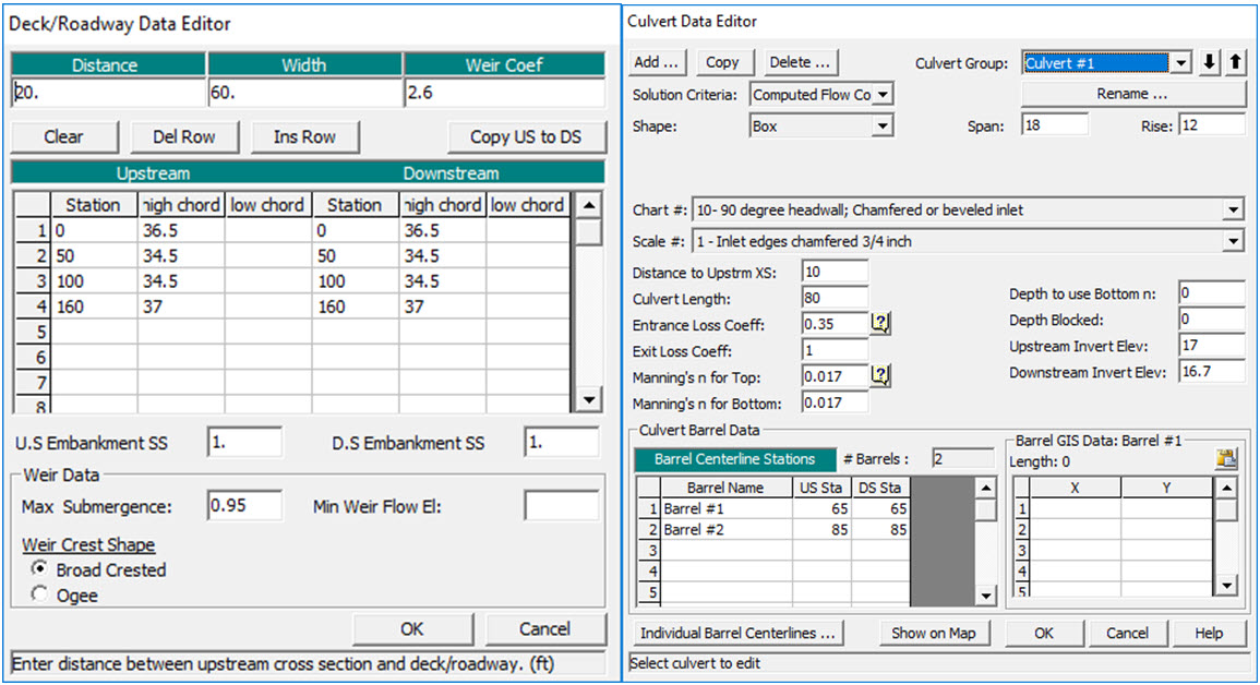
The deck/roadway and culvert editors show the primary culvert input. The deck/roadway data only defines the top-of-road. The low chord is left blank, filling the area from the roadway elevation to the ground.
The culvert data defines the size, shape and location of the culverts. The inlet control is defined by Chart # and Scale. The outlet control information includes culvert length, n value, entrance and exit loss coefficients. The entrance loss coefficient was set to 0.35, halfway between the square and rounded entrance coefficient. The effective area option is input with the bounding cross sections.
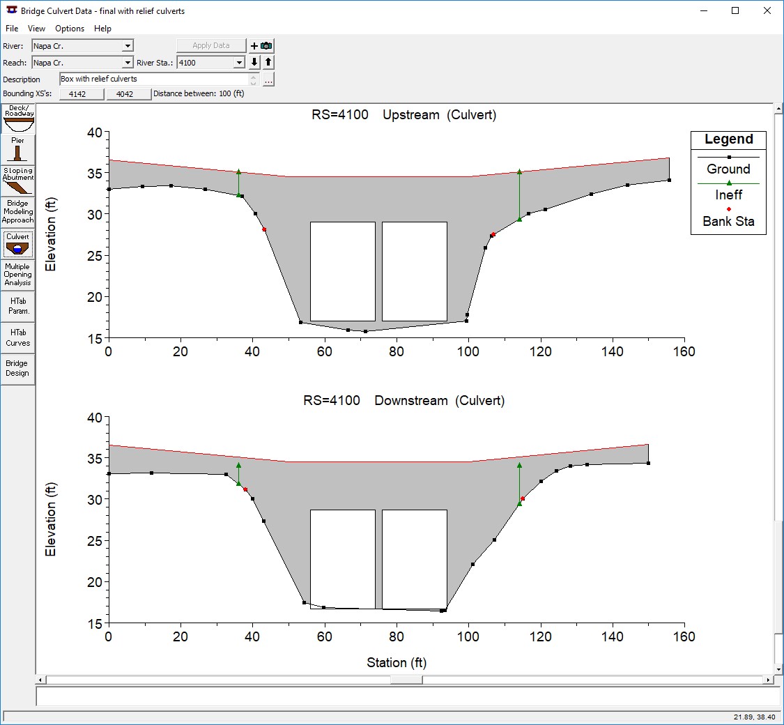
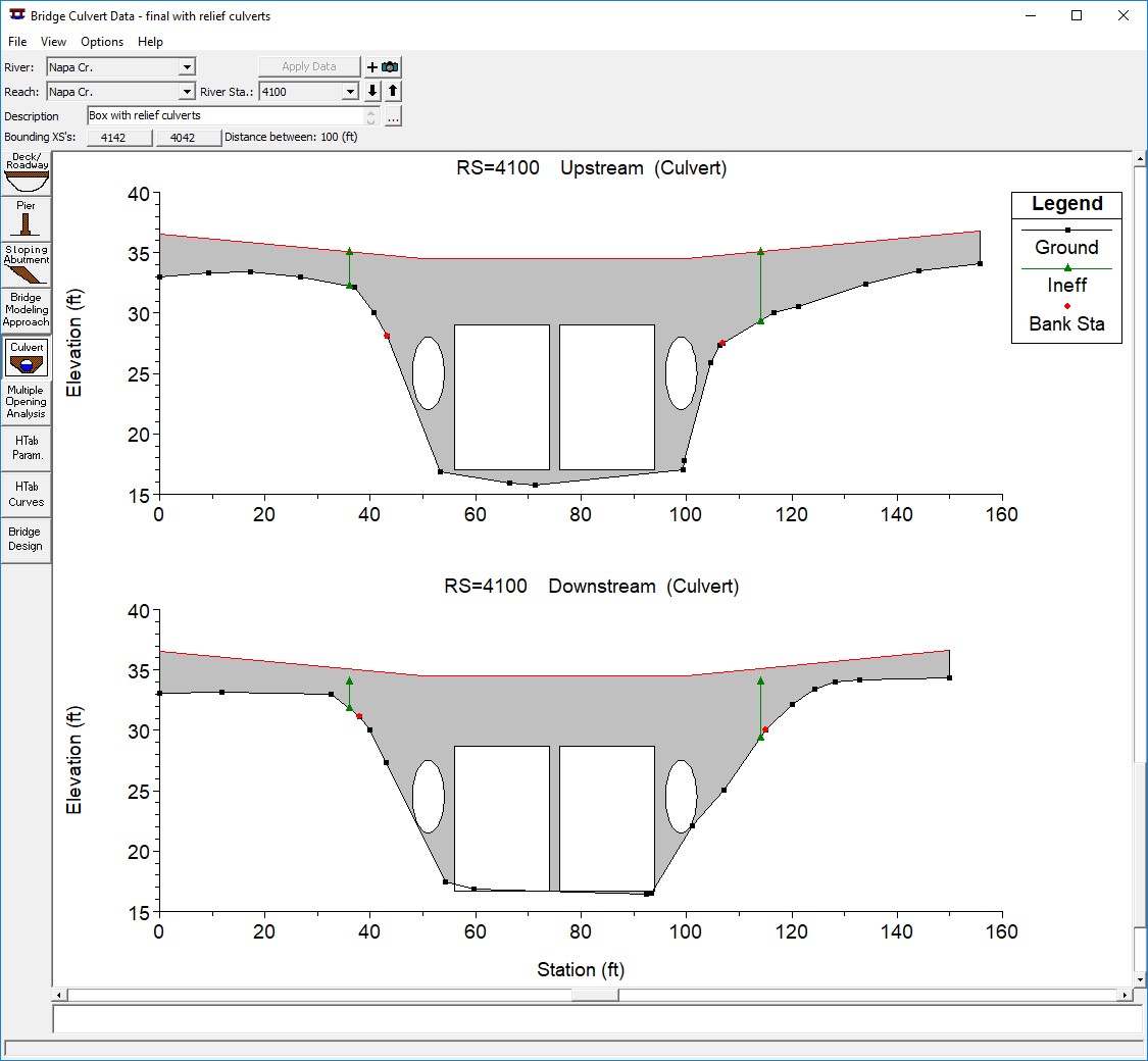
After the data are entered, the Bridge/culvert editor shows the culverts and roadway along with the bounding cross-sectional data. Note the Effective area option is indicated by the green lines with vertical arrows in the display.
- Start a new plan and run the model with the same flow and starting conditions applied to the geometry file with culverts. This will facilitate evaluation.
- Evaluate the model results for completeness and accuracy. Make necessary corrections and run again until satisfied with the results. Then evaluate based on design criteria.
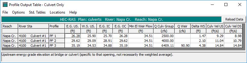
The Culvert Summary Table shows the culvert solution for all profiles. It indicates a small amount of weir flow for the
maximum flow.
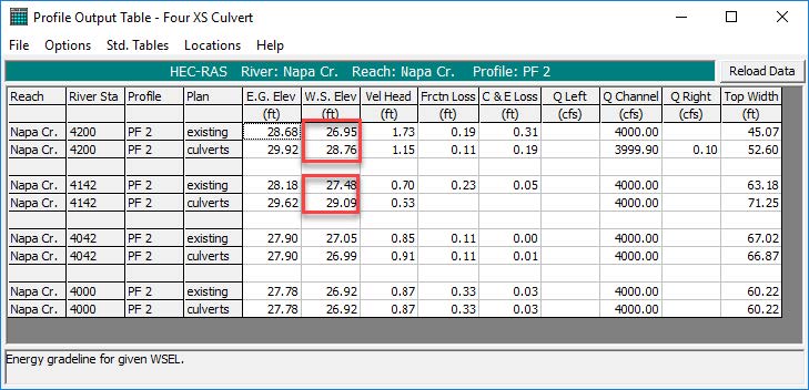
The Four section culvert summary table will show the water surface calculations in the vicinity of the culvert. By requesting the two plans, one can see the differences between the two models. The water is about 1.8' higher at RS 4200.
The Culvert Table, shown under question a, displays inlet and outlet EG. The higher controls; therefore, the solutions are outlet control (E.G.US = E.G.OC) for the first two profiles, and outlet control and weir flow for the third.
Given the outlet control solution, the culvert n value, exit loss and entrance loss coefficients will affect the solution. The values could be easily changed to test the sensitivity of the solution to assumptions of coefficients.
Part 2
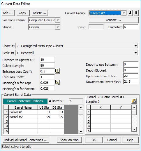
If after completing Part 1 you find that the design criteria are not met, a second option includes adding two corrugated metal culverts to provide added high-flow capacity. Add two 6 foot culverts, one on either side of the box culverts, so they fit within the natural cross section and increase high flow capacity sufficiently to meet the criteria. Assume the added culverts will fit into the 90 degree head wall. Culverts should have a slope of 0.5 feet over their 80 foot length.
Again, be sure to save the new geometry file and run under a new plan label to facilitate comparison between base conditions and the new model.
The culvert data for Culvert group #2 are shown in the editor, adjacent figure. Also, the location of the effective area option was shifted to approximately 10 feet outside of the added culverts. Once the data are entered, the new culverts are displayed in the Bridge editor, as shown below.
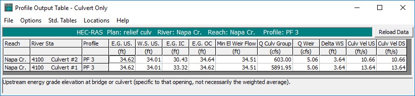
The model was run again with the new geometry. A review of the Culvert Only Table indicates the maximum flood produces a minor amount of weir flow.
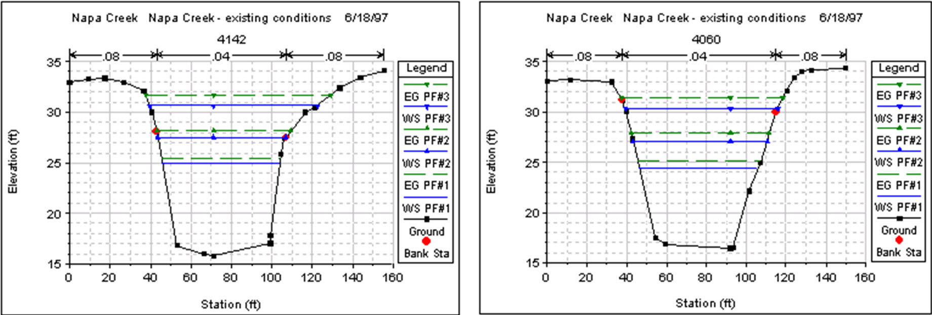
A review of the Culvert cross-section table (see next page) shows this model does not meet design criteria. The relief culverts significantly lower the maximum flood profile and the one-percent chance flood is approximately 1.2 feet (28.18-26.95~1.2) above the base profile at section 4200. The only way to meet the one-foot rise criterion is to lower the losses (e.g., improved inlet) or increase culvert size. Additionally, the maximum profile is still overtopping the roadway. The profile plots, below, show the existing and final model results for the 1 percent chance event.