Steady Flow Modeling with HEC-RAS

Data Files

You will be working with a section of the Merced River at Yosemite, CA.  The data for this tutorial is provided in the zip file.

Steady Flow Modeling with HEC-RAS.zip

Objective

In this workshop, you will learn how to create a 1D model with HEC-RAS of the main channel and floodplain area. This workshop will require you to acquire terrain datasets, create a terrain model, lay out cross sections, provide steady flow information, downstream boundary conditions, add land cover data and associate Manning's n values, refine the model, and perform model runs. You will also attempt to calibrate the model using observed high water mark information using the capabilities in HEC-RAS to adjust Manning's n values.

Background

You will be working on the Merced River in the Yosemite Valley. Steady flow data will be used for the inflow and a Normal Depth Boundary Condition will be used for the downstream boundary.

Create a New RAS Project and Set the Projection

This part of the workshop will guide you through the process of importing terrain data. The terrain data will be used as the basis for the mesh used for 2D hydraulic computations.

1. Start HEC-RAS.
2. Start a NEW project using File | New Project… Go to the workshop directory for this workshop and then provide a Title and File Name. Press OK to save it.
3. Launch RAS Mapper .
4. Select Project | Set Projection. Select the Folder button at the top left and navigate to the "River.prj" provided in the "GIS_Data" folder. Select and Open this file. This sets the coordinate system for all the data you will view in RAS. The press the OK button to close the window.
   
5. Add the "River" shapefile to RAS Mapper from the "/GIS_Data" folder (by dragging and dropping the "river.shp" file onto the Map window).
6. Right-click on the River layer and Zoom to Layer

Download Terrain Data

If you don't have internet access, skip this step and use the terrain data provided in the "Terrain\USGS_Data" folder.

1. Select the Project | Download Data | USGS Terrain menu item.
   
2. Choose Current View for the data's extent.
   
3. Press the Query Products button interrogate the USGS web service.
   
4. Utilize the data filter to Filter to the "Original" data.
   
5. Select the terrain tiles that cover the valley floodplain using the graphical selection tools in RAS Mapper.
   
6. Click the Add Selected button from the Download Terrain dialog.The check boxes will be filled in for the selected datasets and the terrain tiles will turn green (indicating they are selected for download).
   
7. Press the Start Download button. A dialog will inform you when the download is complete.
   
8. Close the Terrain Downloader.

Terrain Model Preparation

1. Import terrain data for use in RAS by selecting the Project | Create New RAS Terrain menu item.
2. Click the Add Files button and navigate to the "Terrain\USGS" folder.
3. Select ALL of the files (Ctrl+A) and then press the Open button at the bottom.
   
4. Click the Merge Inputs to Single Raster checkbox.
5. Press the Create Button.As the Terrain is created, a computation window will inform you of progress.
   
6. When the terrain process is finished, select Close on the processing window, this will close both windows. Turn on the Terrain Layer.
7. Right-click on the Terrain Layer and choose Zoom to Layer (if necessary to see the terrain).
8. Double-click on the Terrain Layer to access its Properties.

Below is what the terrain should look like. Also shown are all the boundary condition locations for this workshop.

Initial Model Creation

In this part of the workshop, you will create the initial model. This rough model will provide and understanding of the floodplain from which you can improve the hydraulics model. The rough model will allow you to answer simple questions such as listed below.

• Where does water go and what is the extent of the floodplain?
• What velocities does the river experience?
• Where is flow rapidly varied?
• What is controlling where flow goes and are there major obstructions to flow?

Create the 1D Geometry

1. Choose the Project | Create New Geometry menu item. Enter "Base" for the name. Press OK to create the geometry layer.
2. Select new Geometry Layer and press the Edit button.
3. Create the River Centerline
   1. Copy and Paste the river centerline from the "River" shapefile (previously loaded) to the River Layer. – or – you could import the river using the shapefile importer. – or – you could create it by hand
   2. Using the Edit tool and right-click on the River line and select Rename River Reach.
   3. Rename the River Reach to "Merced River", "Yosemite Valley".
      
4. Create Cross Sections
   1. Select the Cross Sections layer and lay out cross sections to properly capture the floodplain.
5. Stop Editing and Close RAS Mapper.
6. Open the Geometric Schematic and Open the new Geometry ("Base").
   
7. Stop Editing to Save the Geometry!
8. Enter Manning's n value data
   1. Select the Tables | Manning's n or k values menu item
      
   2. Set all of the n values to 0.04.
9. Open the Reach Lengths data table – notice the Left, Channel, and Right lengths are all the same. Why is that do you think?
10. Close the Geometric Editor.

Enter the Flow Data

1. Open the Steady Flow Data Editior.
2. Enter 6 for the number of profiles.
3. Enter flows of 100, 500, 1000, 2000, 5000, and 10000 cfs.
4. Select the Options | Edit Profile Names menu item and provide names for each flow.
   
5. Enter a Normal Depth boundary condition. What slope should you use? Does it matter?
6. Save the Steady Flow data when complete (call it "Steady Flows").

Plan and Simulation

1. Save a Steady Flow plan ("Base") to use the geometry and flows.
   
2. Run the simulation (press the Compute button).

Set the Bank Stations

You can use a base run to set the bank stations for all the cross sections.

1. After you have run the model, look at the inundation results in RAS Mapper.
2. Plot individual cross sections using the XS Plot in either the main interface or RAS Mapper.
3. Determine which WS Profile looks to be at the channel banks.
4. Open the Geometric Data Editor.
5. Select the Tools | Channel Bank Station Locations menu item.
6. Chose the Profile you decided was at the channel banks.
   
7. Choose how to insert the Bank Stations.
   

Establish Flow Path Lines

If you have time, set up the Flowpaths Layer. If not, skip this step.

1. In RAS Mapper, Edit the Base geometry.
2. Select the Flowpaths Layer and create a flow path line in the left and right overbank.
3. Stop Editing, when finished.

Re-run the Model

1. Compute the Base plan.
2. Evaluate the results.

Model Refinement

Once you have a working model, you can use it to inform you on how to improve/refine the model to better represent real-world conditions. This is where you'd refine the cross section layout, move bank stations, realign flow paths, etc.

Create a Copy of the Geometry

You will want to keep a copy of the old mesh and work on a new one (you never know when you might want to go back, but you will certainly want to compare to see progress).

1. Open RAS Mapper
2. Right-click on the base Geometry and choose Save Geometry As.
3. Provide a new name ("Refined").

Land Cover Data

Utilize the 2019 NLCD dataset provide for you to compute hydraulics using spatially varied Manning's n Values.

1. Choose the Project | Create New RAS Layer | Land Cover Layer
2. Select the NLCD_2019.tif file from the "GIS_Data" folder.
   
3. Press the Create button
4. Close the compute window when finished.
5. Associate the LandCover layer with your geometry, in the dialog that appears.
   

Manning's n values

1. Right-click on the LandCover layer and select Edit Land Cover Data Table to associate Manning's n value data with the classification scheme.
   
2. Provide base Manning's n values in the table provided.
   
3. Update the Cross Sections with Manning's n values for the cross sections.
   1. Start Editing the new Geometry
   2. Select the Cross Section Layer and choose the Update Cross Sections | Manning's n Values menu item.
      
   3. You can see if it worked by turning on the Cross Section Layer Plot Option | Manning's n Values.
   4. Stop Editing and Save Edits.

Plan and Simulation

1. Open the Steady Flow Analysis window and create a new Plan using the refined geometry using the File | Save Plan As menu option.
2. Provide a new Title and Name ("Refined").
3. Make sure to select the Refined geometry.
   
4. Run the simulation (press the Compute button).

Evaluate/Compare Results

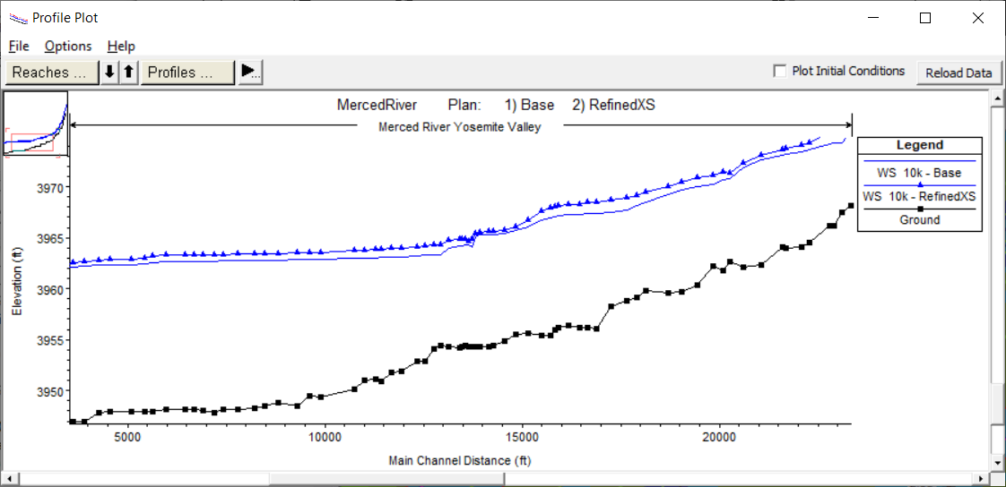
Plot the Water Surface Profile Results comparing the two plans.

1. Plot them using the Profile Plot
   1. Compare plans by selecting the Options | Plans menu item.
   2. Turn on the both plans
      
2. Plot them in RAS Mapper
   1. Select the River centerline layer you added at the start of the project. Right-click on the line and choose Save as Profile Line. Provide a name.
   2. Turn on the WSE layer for both results
   3. Highlight the Results group layer, press the Max button on the Animation control.
   4. Click on the Profile Lines tab (lower left corner).
   5. Right-click on the River line and select the Plot Profile | WSE menu item

Observed Data

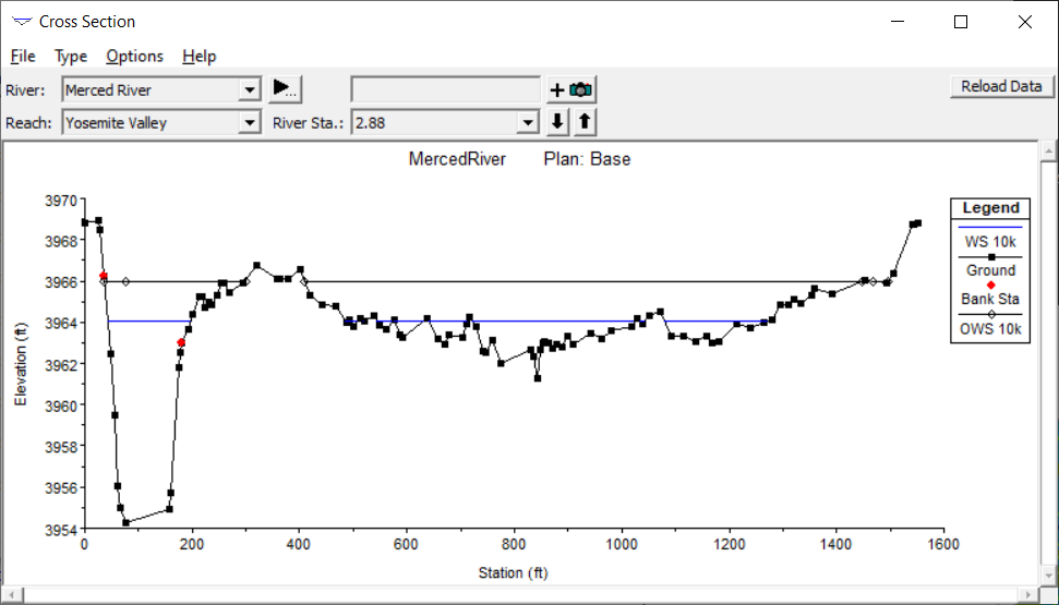
At this point we don't really know how are model is doing. We can use observed data to help inform us and how to refine the model. Add an Observed High Water Mark (at the Bridge, at the Yosemite Falls Vantage Point, near River Station 2.88 based on the provided river centerline).

1. Open the Steady Flow Data editor.
2. Select the Options | Observed WS menu item.
3. Select the river station 2.88 (yours may vary) and Add the Observed WS Location.
   
4. Enter a WSE of 3966ft for the 10,000cfs profile.
5. Save, and Close the Unsteady Flow Editor
6. Re-run the simulation

 Improve Manning's Data

1. Select the LandCover | Classification Polygons layer
2. Start Editing
3. Right-click on the Classification Polygons and choose the Import Features from Shapefile menu option
4. Select the "Channel_Polygon" shapefile in "GIS_Data" folder.
5. Switch to the Edit Tool and then right-click on the new channel shape and choose Edit Classification Value.
   
6. Enter a value of 0.04 for the Manning's n value.
   
7. Stop Editing and Save edits.
8. Update the Cross Sections with Manning's n values for the cross sections.
   1. Start Editing the new Geometry
   2. Select the Cross Section Layer and choose the Update Cross Sections | Manning's n Values menu item.
   3. Stop Editing and Save Edits.
9. Re-run and Compare results.

Sensitivity Analysis – Bonus Material

As time allows perform sensitivity analysis.

1. How sensitive is the model to the downstream boundary?
2. What do the model results show if you increase or decrease the Manning's n values?