Troubleshooting with HEC-RAS

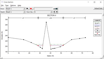
This problem initially runs.  However, while reviewing the output for this problem, it was noted that at cross section 4.0 a subcritical water surface could not be computed.  The program defaulted to critical depth at this location (as shown below) and then continued on upstream.

A cross section plot of river station 4.0 (shown below) shows that the cross section has a point in the middle of the main channel that is much higher than all the data points.  Review of the cross sections immediately upstream and downstream of this section, show that this data point is not realistic and was probably entered incorrectly.

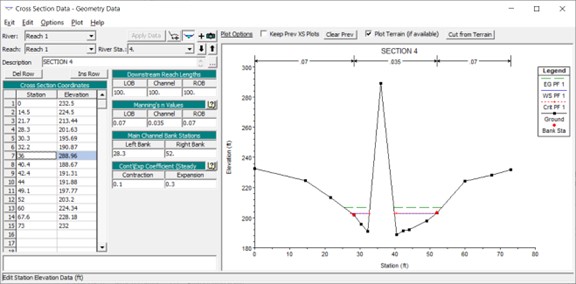
To fix the problem the cross section editor was opened and cross section 4.0 was loaded.  As shown below, cross section station 36 had an elevation of 288.96.  The elevation seems to 100 feet higher than it should be.  This probably was a keypunch error when the data was being entered. 

The data point was changed to 188.96, and the file was saved.   The profile was re-computed, and the results showed that all cross sections were subcritical. 

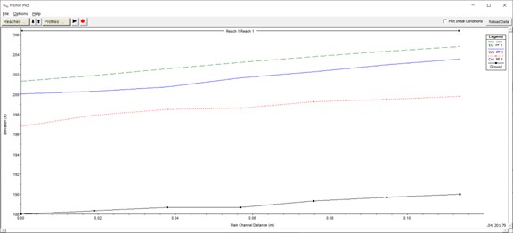
The resulting water surface profile after the data entry correction is shown below.

While reviewing the output for this problem, is was noted that both profiles went to critical depth at river station 4.0.  The figure below shows the profiles for this problem.

Further review of the “Errors, Warnings, and Notes” show that every cross section is getting the following message:

Warning - The energy loss was greater than 1.0 ft (0.3 m). between the current and previous cross section.  This may indicate the need for additional cross sections.

In addition to this message, several cross sections were also getting the following messages:

Warning - The velocity head has changed by more than 0.5 ft (0.15 m).  This may indicate the need for additional cross sections.

Warning - The conveyance ratio (upstream conveyance divided by downstream conveyance) is less than 0.7 or greater than 1.4.  This may indicate the need for additional cross sections.

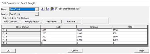
Reviewing the cross section plots does not show any significant problems with the data.  Reviewing the input data for the cross sections reveals that the cross section reach lengths seem very far apart. A table of reach lengths from the geometric data editor is shown below.  As shown in the table, most of the reach lengths are well over 1000 feet.  This specific reach is also relatively steep, with an elevation change of around 19.0 feet over approximately one mile.  Given the steepness of the reach; the long reach lengths; and the Warning messages; it appears that the main problem is that there are two few cross sections for this length of stream.

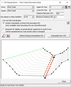
The best solution to this problem would be to get additional surveyed cross section data.  If this is not possible, or not affordable, another possible solution is to use the HEC-RAS cross-section interpolation routines to supplement the data.  For this data set, cross-sections were interpolated every 100 feet based on the main channel reach lengths.  The cross sections were interpolated using the “Within A Reach” interpolation option from the Geometric Data Window.  Once the cross sections are interpolated, the user should always review the interpolated cross sections to make sure the interpolation is reasonable.  The best way to do this is to use the “XS Interpolation - Between 2 XS’s” option.  This allows you to view previously interpolated cross sections, and to re-interpolate any sections that do not look reasonable.  The figure below shows the Interpolation between sections 3 and 4.

Once the cross section interpolation was finished, the data was saved and the water surface profiles were computed.  The figure below shows the new water surface for profile 2, with the interpolated cross sections.

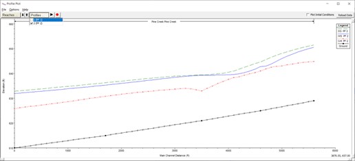
As shown in the figure above, the water surface is subcritical throughout the reach.  In addition, all of the warning messages are gone except two.  The two remaining messages state that the velocity head has changed by more than 0.5 feet at two of the cross sections.  Closer review at these two locations shows that it is not a problem, and therefore the messages can be ignored.  The new water surface profiles are smooth and appear to be greatly improved over the original run.

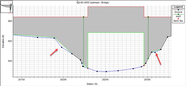
This data set has five cross sections.  Each cross section has the levee option turned on for either the right or left overbank, and section two has it for both overbanks.  The overbank areas of the stream are lower than the main channel bank stations, and the levee option keeps water from going out there until the levee elevations are exceeded.

Review of the output for this data set shows that the water surface was for the most part contained within the main channel, except at cross section 2.0.  At this cross section, the water surface was just above the levee elevations on both the right and left banks.  Because of this, cross section two shows significant amounts of flow in both the left and right overbanks, while all the other cross sections do not.  This is not a realistic answer.  The question is, how much water will actually go over the levees into the overbanks, and will it completely fill the overbank areas.  Since HEC-RAS is being run in a one-dimensional flow mode, it can only calculate a single water surface.  While in reality, the water surface could be higher in the main channel than in the overbanks.   In addition to that, if a significant amount of water does get out into the overbanks at cross section 2.0, then there will probably be water out into the overbanks at the cross sections downstream of section 2.0. 

One approach to this problem is to maintain all of the flow in the channel and determine what the resulting water surface profile would be (this will give the maximum profile height).  This was accomplished by raising the levee elevations slightly for cross section 2.0.  Figure 9 shows the resulting water surface at cross section 2.0 with the levees raised.  The output for this run results in a water surface elevation of 18.82 feet at section 2.0.  The original run had a water surface elevation of 18.62 feet.  The true tops of the left and right overbanks are 18.5 and 18.2 feet respectively.

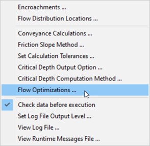
Obviously, some water is going to spill out into the overbanks.  The amount could be estimated by applying a weir equation to the overbank profiles.  Once the weir flow is estimated, the flow downstream could be reduced to reflect the lost water.  HEC-RAS provides a lateral structure option that can model the levee profile as a weir.  Then, under the Steady Flow Options, the Flow Optimization feature can be applied to compute the flow loss and the resulting water surface profile.

Another aspect that should be considered is the duration of the peak flow. This will be important in estimating the volume of water getting out into the overbank area.  The solution to this problem is to compute an unsteady flow profile with the full flood hydrograph.

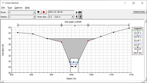
Problem number 4 is a short reach of stream with a single box culvert crossing at river station 2.5.  While reviewing the output, it was found that the water surface goes to critical depth just upstream of the culvert, for both profiles.  The profile plot (shown below) looks especially strange, with the culvert barrel and critical depth inside the culvert appearing to be below the channel invert on the upstream side.

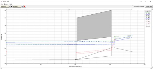
Further review of the data shows that the upstream end of the culvert has been entered at an elevation below the invert of the upstream cross section.  The figure below, shows a cross section plot of the upstream end of the culvert.  As shown in figure, the culvert is about two feet below the upstream cross section.  Either the culvert is not at the correct elevation, or the upstream cross section does not correctly reflect the culvert opening.  The result is that the program can correctly compute the energy loss through the culvert, but when that energy is placed into the upstream cross section, there is not enough available area to obtain a subcritical water surface.  Therefore, the program defaults to critical depth.

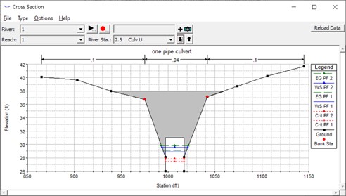
Assuming that the data for the culvert is correct, the solution to this problem is to modify the upstream cross section to include the area of the culvert.  Using the cross section editor, cross section 3.0 was modified, and the profiles were re-computed.  The figure below shows a cross section plot of the upstream end of the culvert, for the modified data.

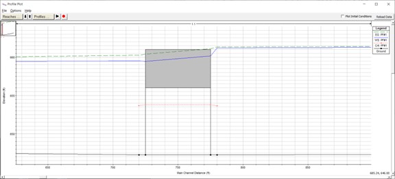
The resulting water surface profiles for the revised run is shown in the figure below.  As shown in figure, the profiles remain subcritical through the culvert and upstream of the culvert.  The graphic no longer shows critical depth inside the culvert being below the upstream cross section invert elevation.

While reviewing the output, at first glance it looks like there are no major problems with this data set.  However, closer review of the output shows some peculiarity in the water surface at the bridge.  While viewing the water surface profile, a zoomed in view around the bridge shows the water surface going through the deck (see figure below).

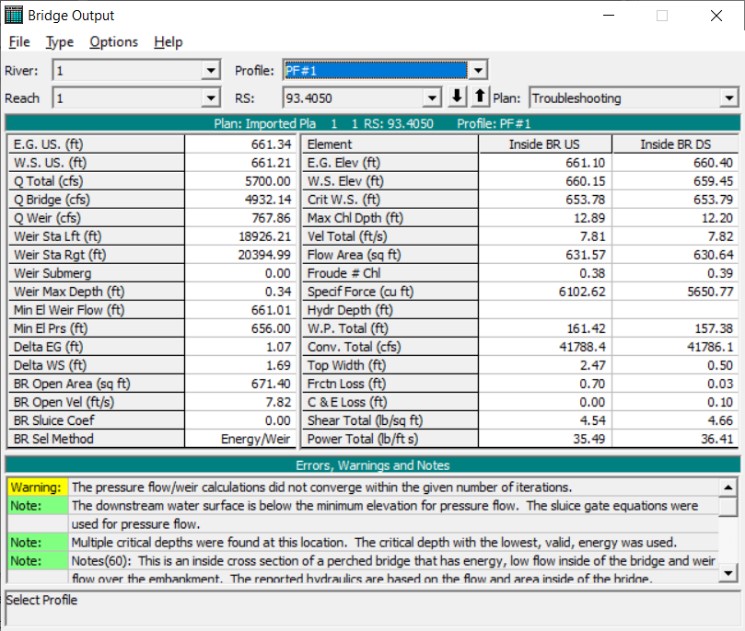
The selected high flow bridge modeling approach is “Pressure and Weir” flow. Further review of the bridge results shows that the program selected a solution of “Energy only” flow, and the notes list warns that the pressure/weir flow calculations did not converge.  The detailed bridge table showing the final bridge solution at the lower left part of the table (shown here).   The solution of Energy only flow means that the energy equation was used for the low flow and the high flow through the bridge opening.  This solution does not seem consistent with the selected bridge modeling approach and the physical representation of the bridge.

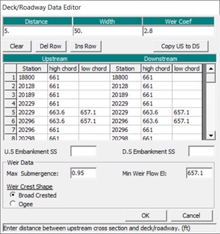
While reviewing the bridge input data, the graphic of the bridge shows some gaps between the bridge deck and the ground.  The figure below shows a zoomed in view of the upstream side of the bridge.

As highlighted in the figure, gaps between the bridge deck and the ground can cause the program to compute incorrect hydraulic parameters (too much wetted perimeter and area) as well as arriving at an inconsistent modeling solution.  Sometimes these mistakes can even cause the program to “blow up” (stop running) during the bridge computations.  To assist the user in finding geometric mistakes in bridges and culverts, an option called “Highlight Weir, Opening Lid and Ground” is available from the View menu of the Bridge and Culvert data editor.  This option will highlight the important parts of the bridge opening.

The first is the weir profile, which will be highlighted in red.  The weir profile represents the combination of the high ground information and the high cord elevations of the bridge deck/roadway data.  This information will be used as the weir profile if you choose to model the bridge as pressure and weir flow.  Otherwise, if you use the energy method for high flows, this will simply be used as additional flow area and wetted perimeter.  The next highlighted line will be the bridge opening “Lid”, which will color in green.  This represents the top of the bridge opening.  The last highlighted line will be the bridge opening “Ground”, which will be colored in blue.  This represents the bottom of the bridge opening.  When you turn this option on, any openings that should not be there will show up more readily.  Additionally, other types of geometric mistakes can be diagnosed if the three lines do not appear to be correctly depicting the weir profile and bridge opening.

The solution to this example is to edit the bridge Deck/Roadway data in order to get rid of the gaps between the deck/roadway and the ground.  The main problem is that the low chord information should be entered below the natural ground profile.  The program will automatically clip off any excess below the ground stations.  An additional problem in this data set is that the Deck/Roadway data was entered starting at the very left end of the cross section data; following the ground profile in the left overbank; then across the main stream; and again following the ground profile in the right overbank.  This is not necessary in HEC-RAS.  It was originally necessary in the HEC-2 program in order to allow the overbank area to be modeled as part of the weir.  But in HEC-RAS it is only necessary to model the additional area that must be blocked out due to the actual road embankment and bridge data.

The Deck/Roadway data was modified to reflect the changes discussed above.  The figure below shows the Deck/Roadway data editor with the modified data loaded.

If the low chord is going to intersect the ground, it is better to leave the data blank and allow RAS to “take it to the ground”.

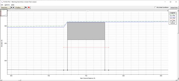
Once the new data was entered, the program was re-run and a solution of Pressure/Weir flow was arrive at.  A review of the output showed the results to be reasonable, with the possibility of some minor problems with cross sections spacing.  The figure below shows a profile plot of the new solution.

This problem is a short reach of river with a bridge at river station 6.15.  Upon review of the output no computational problems can be found.  In addition, the errors, warnings, and notes messages do not imply that there are any significant problems.  However, while looking at the cross section plots for the bridge, it can be seen that in the vicinity of the bridge, there is an area in the right overbank that is lower than the bridge deck.  The second and third profile shows water out in this low area.  In addition, the third profile has highly submerged the bridge.  A plot of the bridge cross-section and the three profiles is shown below.  Reviewing the modeling approach for this bridge shows that it was modeled with the pressure and weir flow option for high flows.

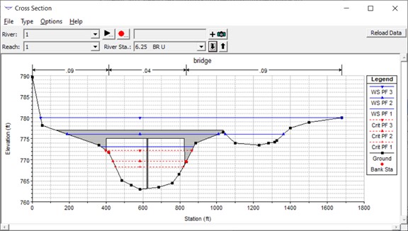
Given that the bridge deck is not very thick (only about 2 feet), and there is an area in the right overbank in which the flow can go around the bridge without the bridge being overtopped, it is not likely that this bridge will act like a true pressure orifice and a weir.  In the third profile, the water surface is far above the top of the bridge.  While reviewing the bridge specific table for the third profile, it can be found that the flow going over the top of the road (i.e. the weir) was submerged by 85 percent. 

A couple of possible solutions could be used on this problem.  One is that the bridge could be modeled as a multiple opening, with a bridge opening and an open channel flow area (conveyance area) in the right overbank.  The bridge may still be modeled as pressure and weir flow in this case.

A second solution would be to assume that the bridge itself is not going to block a significant amount of the flow area (especially for the third profile), and therefore it may be better to model this bridge with the energy method for high flows.  The modeling approach was switched to the energy method for high flows, and the profiles were re-computed.  The results for the two runs are shown in the table below.

Energy and Pressure/Weir Results