Download PDF
Download page 2D Model Development and Refinement.
2D Model Development and Refinement
Data Files
You will be working on the Merced River in the Yosemite Valley. Data files for this tutorial are provided in the zip file.

Objective
In this workshop, you will learn how to create a 2D HEC-RAS model of a main channel and floodplain area. This comprehensive workshop will require you to create a terrain model, develop a 2D mesh, provide inflow hydrograph information, downstream boundary conditions, add land cover data and associate Manning's n values, refine the model using breaklines, and perform model runs. You will also attempt to calibrate the model using observed high water mark information using the capabilities in HEC-RAS to adjust Manning's n values.
Background
You will be working on the Merced River in the Yosemite Valley. A flow hydrograph will be used for the inflow and a Normal Depth Boundary Condition will be used for the downstream boundary.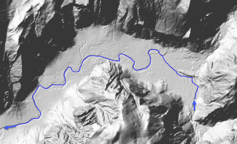
Create a New RAS Project and Set the Projection
This part of the workshop will guide you through the process of importing terrain data. The terrain data will be used as the basis for the mesh used for 2D hydraulic computations.
- Start HEC-RAS.
- Start a NEW project using File | New Project… Go to the workshop directory for this workshop ("Merced River") and then providing a Title and File Name. Press OK to save it.
- Launch RAS Mapper
 .
. - Select Project | Set Projection. Select the Folder button at the top left and navigate to the "River.prj" provided in the "GIS_Data" folder. Select and Open this file. This sets the coordinate system for all the data you will view in RAS. The press the OK button to close the window.

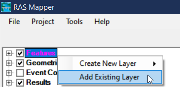
- Add the "River.shp" file to the RAS Mapper by right-clicking the Features Node in the tree and selecting "Add Existing Layer".
- Right-click on the River layer and Zoom to Layer
Download Terrain Data
If you don’t have internet access, skip this step and use the terrain data provided in the “Terrain\USGS_Data” folder.
- Select the Project | Download Data | USGS Terrain menu item.

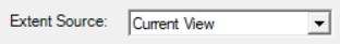
- Choose Current View for the data’s extent.
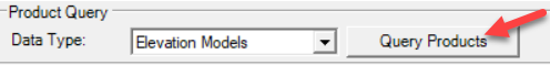
- Press the Query Products button interrogate the USGS web service.
- Utilize the data filter to Filter to the “Original” data.

- Select the terrain tiles that cover the valley floodplain using the graphical selection tools in RAS Mapper.
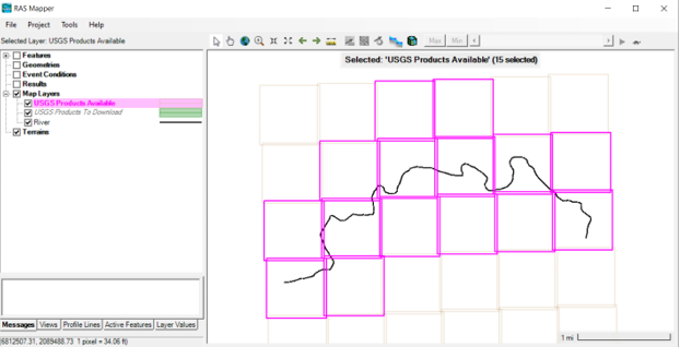
- Click the Add Selected button from the Download Terrain dialog.
The check boxes will be filled in for the selected datasets and the terrain tiles will turn green (indicating they are selected for download).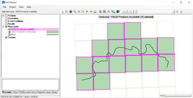
- Press the Start Download
A dialog will inform you when the download is complete.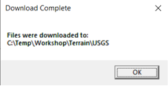
- Close the Terrain Download dialog.
Terrain Model Preparation
- Import terrain data for use in RAS by selecting the Project | Create New RAS Terrain menu item.
- Click the Add Files
 button and navigate to the "Terrain\USGS" folder.
 - Select ALL of the files (Ctrl+A) and then press the Open button at the bottom.
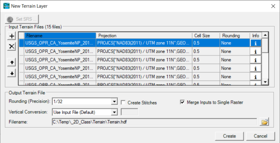
- Click the Merge Inputs to Single Raster checkbox.
- Press the Create Button.As the Terrain is created, a computation window will inform you of progress.
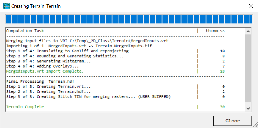
- When the terrain process is finished, select Close on the processing window, this will close both windows. Turn on the Terrain Layer.
- Double-click on the Terrain Layer to change the Display Properties to your preference.
Initial Model Creation
In this part of the workshop, you will create the initial model. This rough model will provide and understanding of the floodplain from which you can improve the hydraulics model. This type of rough model will allow you to answer simple questions such as listed below.
- Where does water go and what is the extent of the floodplain?
- What velocities does the river experience?
- Where is flow rapidly varied?
- What is controlling where flow goes and are there major obstructions to flow?
Create the 2D Flow Area
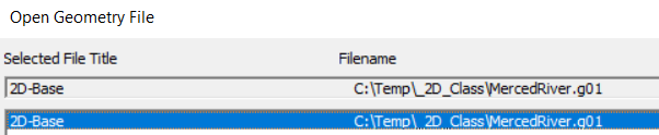
- Choose the Project | Create New Geometry menu item. Enter "2D – Base" for the name. Press OK to create the geometry layer.
- Select new Geometry Layer and press the Edit button.
- Select the 2D Flow Areas Perimeter layer (you will need to expand the layer tree). Draw the perimeter using the Add New Feature
 tool.
tool. 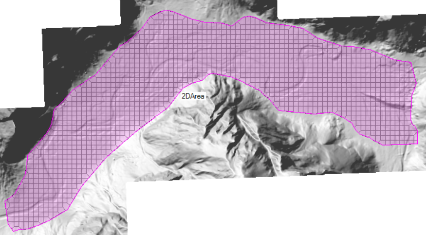
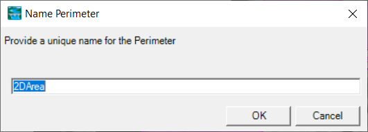
- Enter a name, when finished.
- In the Edit 2D Area Properties that come up, Enter 200 for the DX and DY Point Spacing.
- Click on the Generate Computation Points button.
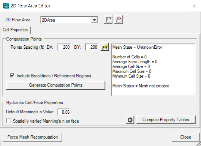
- Close the Editor.
- Turn on the Computation Points.
- Stop Editing to Save the Geometry!
Boundary Conditions
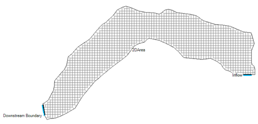
After creating the 2D Flow Area computation mesh, add boundary conditions.
- Edit the Boundary Condition Lines Layer.
- Draw external boundary conditions, left to right when looking downstream at the Inflow and Downstream Boundary locations.

External Boundary Conditions must be drawn outside of the perimeter of the mesh.
- Stop Editing and Close RAS Mapper.
- Open the Geometric Schematic and Open the new Geometry ("2D - Base"). This allows the unsteady flow file to get the boundary condition locations.
- Close the Geometric Editor.
Unsteady Flow Editor
- Open the Unsteady Flow Data editor and enter boundary condition information.
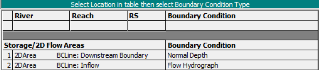
- Use Normal Depth with Slope = 0.001 for the downstream boundary condition.
- Use the "streamflow.dss" file to define the Flow Hydrograph for the upstream boundary and tributaries. You will need to click the Add DSS File
 button to add the DSS file prior to picking a path.
 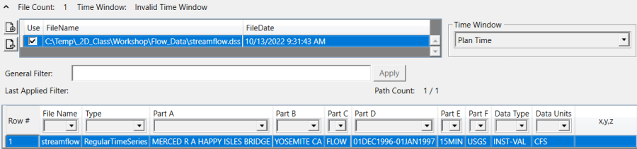 The hydrograph for the inflow is USGS 15min data at the Happy Isles Bridge.
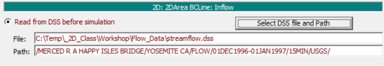
- Specify the "EG Slope for distributing flow along BC line" as 0.01. (This is located at the bottom right on the Flow Hydrograph window.)
- Save the Unsteady Flow data when complete (call it "1997 Flood").
Plan and Simulation
- Save a plan ("Initial").
- Open the Unsteady Flow Analysis window, Save a Plan, and enter all of the necessary information to make a run.
- Set up the time window:
Start Date: 31DEC1996
Start Time: 0000
End Date: 05JAN1997
End Time: 0000 - Turn on the Geometry Preprocessor and Unsteady Flow Simulation programs.
- Specify a computation Time Step and other output options.
So you have to ask yourself two questions (1) What is my cell size? and (2) What velocities do I expect to see?
We have a cell size of 200ft. We can expect normal river velocities of ...5 ft/s...give or take. So we if are to to satisfy a Courant number of 1, a 40 second timestep is 'required". If we relax that a bit, 1 minute timestep should be fine. After you run the model for the first time, you can see if your initial guess on the velocity was correct.
- Compute the simulation.
Manning's Data Improvement
Once you have a working model, you will spend a great deal of time refining the model to represent real-world conditions. In this iteration you will improve upon the roughness values in the model.
Create a Copy of the Geometry
You will want to keep a copy of the old mesh and work on a new one (you never know when you might want to go back, and you will certainly want to compare to see progress).
- Open RAS Mapper
- Right-click on the base Geometry and choose Save Geometry As.
- Provide a new name ("Improved").
Land Cover Data
Utilize the 2019 NLCD dataset provided for you to compute hydraulics using spatially varied Manning's n Values.
- Choose the Project | Create New RAS Layer | Land Cover Layer
- Select the NLCD_2019.tif file from the "GIS_Data" folder.
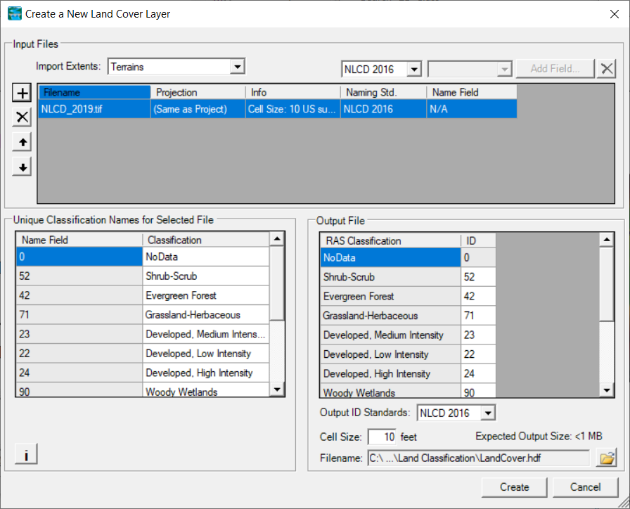
- Press the Create button
- Close the compute window when finished.
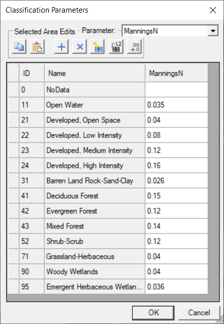
- Right-click on the LandCover layer and select Edit Land Cover Data Table to associate Manning's n value data with the classification scheme.

- Provide base Manning's n values in the table provided (sorting by ID will be helpful).
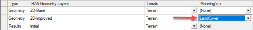
- Choose Project | Manage Layer Associations and associate the LandCover Layer with the new Geometry.
- Start Editing the new Geometry
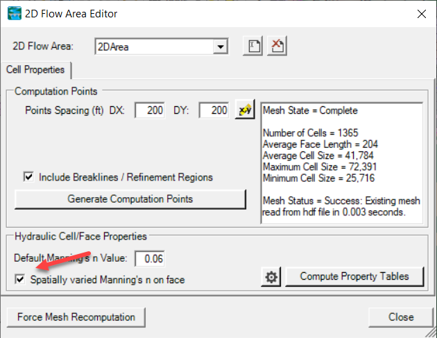
- Edit the 2D Flow Area Perimeter using the Edit 2D Area Properties
- Turn on the Spatially varied Manning's n on face option.
- Stop Editing
Plan and Simulation
- Open the Unsteady Flow Analysis window and create a new Plan using the refined geometry using the File | Save Plan As menu option.
- Provide a new Title and Name ("Improved").
- Make sure to select the Improved geometry.

- Compute the simulation.
Evaluate/Compare Results
- Select the River centerline layer you added at the start of the project. Right-click on the line and choose Save as Profile Line. Provide a name.
- Turn on the WSE layer for both results
- Highlight the Results group layer, press the Max button on the Animation control.
- Click on the Profile Lines tab (lower left corner).
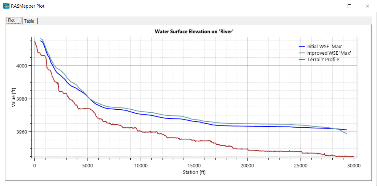
- Right-click on the River line and select the Plot Profile | WSE menu item
The water surfaces are significantly different. Despite using a base n value of 0.06 for the Initial run, the water surface is higher for the NLCD dataset.
If we look at the n values, we can see that the NLCD data is not very good. We have n values of 0.12 in the main channel. That is not good.
Reference Points
At this point we don't really know how our model is doing. We can use observed data to help inform us and how to refine the model. Add a Reference Point at the Yosemite Falls Vantage Point.
- Start Editing the Improved Geometry
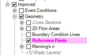
- Select the Reference Points layer
- Right-click and choose the Import Features From Shapefile menu option.
- Select the ReferencePoints shapefile from the "GIS_Data" folder.
- Import the Reference Point.
- Stop Editing and Save Edits.
- Open the Unsteady Flow Data editor.
- Click on the Observed Data tab.
- Click the Edit button in the Observed Stages group.
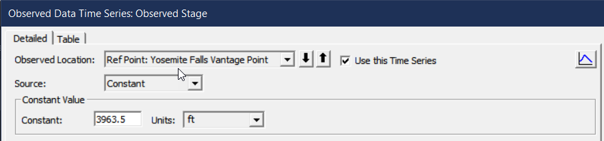
- Choose the Reference Point "Yosemite Falls Vantage Point"

- Choose the Constant for the Source value.
- Enter the observed High Water Mark Elevation of 3963.5ft.
- Click OK, Save, and Close the Unsteady Flow Editor
- Re-run the simulation
- In RAS Mapper, evaluate the computed water surface at the Reference Point. This will require you to
- Expand the "Improved" results group and then expand the Geometry node
- Select the Results (or Reference Point) Layer
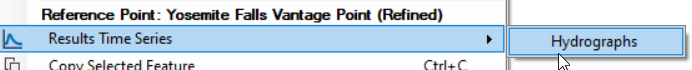
- Right-click on the Reference Point and choose the Results Time Series | Hydrograph menu item.
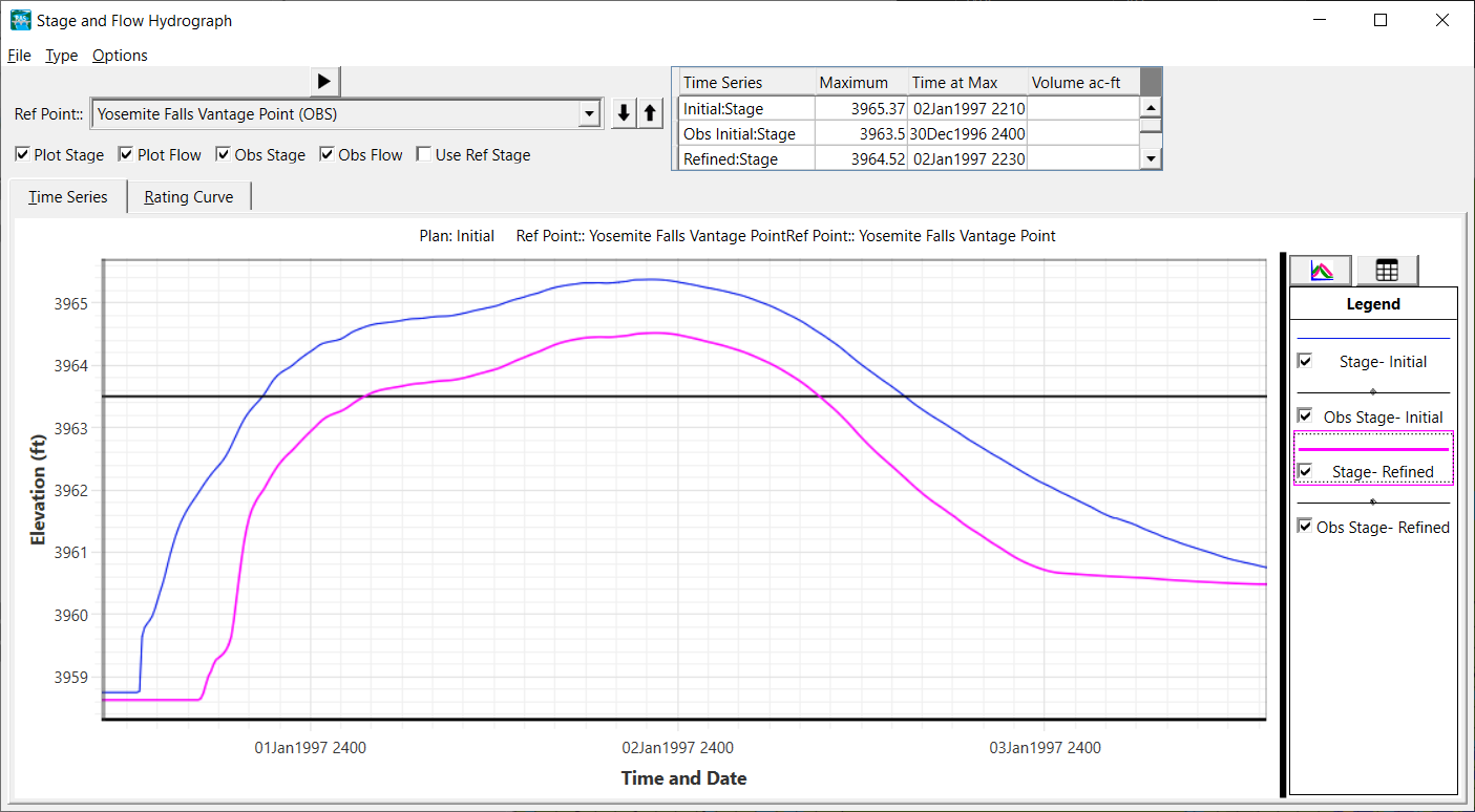
- You can add both Plans to the plot.
- Expand the "Improved" results group and then expand the Geometry node
They are significantly different. Again, the Improved run is higher than the Initial run (and not really improved!).

We need to define better n values. Putting in a realistic value for the main channel will help a great deal.
Lets do that next!
Further Improve Manning's Data
- Select the LandCover | Classification Polygons layer
- Start Editing
- Right-click on the Classification Polygons and choose the Import Features from Shapefile menu option
- Select the "Channel_Polygon" shapefile in "GIS_Data" folder.
- Switch to the Edit Tool and then right-click on the new channel shape and choose Edit Classification Value.
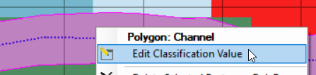
- Enter a value of 0.04 for the Manning's n value.
- Stop Editing and Save edits.
- Re-run and Compare results.
The refinement of the channel n value helped improve the solution, when compared with the observed high water mark.
Model Refinement with Breaklines
There are many roads/high ground that control flow in this domain. Use breaklines to improve the model. In addition to breaklines, think about ALL of the ways you can improve the model!
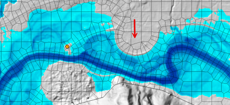
Note: the Visitors Parking lot east of the Reference Point should NOT be wet.
Create a Copy of the Geometry
- Open RAS Mapper
- Right-click on the Improved Geometry and choose Save Geometry As.
- Provide a new name ("2D-Refined").
Add Breaklines
- Start Editing the Refined Geometry
- Click on the Breaklines layer.
- Add Breaklines, as appropriate. Use a 100ft spacing for breaklines.
- Fix the mesh if errors occur!

- Stop Editing and save edits.
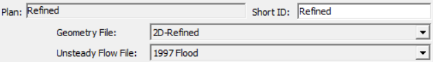
- Open the Unsteady Flow Analysis window and create a new Plan using the refined geometry using the File | Save Plan As menu option.
- Provide a new Title and Name ("Refined").
- Make sure to select the Refined geometry.
- Select an appropriate Time Step and Compute the simulation.
Adding breaklines to high ground is the correct way to align faces for 2D modeling in HEC-RAS. Adding breaklines to the road network and other high ground improves the mapping a great deal. The parking lot is now dry.
We can always spend more time refining cells, adding breaklines, and improving Manning's n value data. It is important to have observed data to calibrate to when spending time refining a model. Further, hydraulic structures such as bridges should be included in the model. If velocity results were important, we would need to reduce 2D cell sizes!
Bonus Material- Sensitivity Analysis
As time allows perform sensitivity analysis. Investigate the following items below.
- How sensitive is the model the equation set selected?
- What do the model results show if you increase or decrease the Manning's n values?
- Do the results differ if you add more cells in the channel?
- How are your run times being impacted?