Download PDF
Download page Combined 1D2D Modeling.
Combined 1D2D Modeling
Data Files
You will be working with a section of the Bald Eagle Creek river near Lock Haven, PA. Data files for this tutorial are provided in the zip file.

Objective
In this workshop, students will use HEC-RAS to:
- Model areas behind levees with 2D Flow Areas
- Attach 2D Flow Areas to 1D Cross Sections using a Lateral Structure
- Compare and understand differences between 1D and 2D approaches
Background
The town of Lock Haven is situated on the north bank of Bald Eagle Creek in central Pennsylvania. Lock Haven is protected by a levee system that was designed to provide for a 500-year (0.2% Chance) event. Sayers Dam, a flood control project on Bald Eagle Creek, is approximately 15 miles upstream of Lock Haven. See the figures below to become acquainted with the domain.
In this workshop we will analyze how the levees perform for a 1000-year event and compare difference in results between 1D and 2D approaches for modeling the protected area.


Review 1D Results
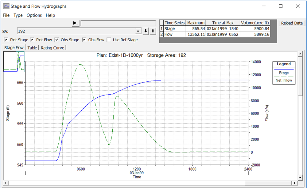
- Open the Project and Run the 1D Plan called "Existing Conditions 1D – 1000 yr Event".
- Review the model results. Specifically, look at the water surface profiles and hydrographs to see what is happening around the town of Lock Haven.
In general, the Hydraulic results look reasonable. The levees get overtopped at the upstream end of the system. The 1000 yr event overtops the levee system and fills the interior areas with a significant amount of water.
However, when the levees are first overtopped the interior areas get filled from the low point in the storage areas first, and they fill up as level pools. This is not as accurate as it could be for estimating arrival times at various locations in the Lock Haven area.

Replace 1D Elements with 2D Flow Area
- Go to RAS Mapper and make a copy of the current Geometry data using the Save Geometry As option.
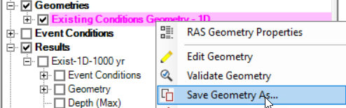
- Name the new geometry something like: "Existing – 2D Levee Area"

- Start Editing the geometry
- Storage Areas layer - Delete the Storage Areas labeled 191 and 192 (the two upstream).

- SA/2D Connections layer - Delete the hydraulic connection that was between storage areas 191 and 192
- Import the new 2D Flow Area perimeter

- Click the browse icon, navigate into the "GIS_Data" folder and select "LockHaven2DPerimeter.shp". You should see your perimeter now in the Importer.

- Click Import, and your 2D perimeter will load into the geometry.
- Click the browse icon, navigate into the "GIS_Data" folder and select "LockHaven2DPerimeter.shp". You should see your perimeter now in the Importer.
- Create a mesh for the new 2D Flow Area
- Right-click on the "Perimeters" layer in the map window and select Edit 2D Area Properties

- Create the 2D Mesh with 100ft cell spacing and Manning's n value of 0.06.

- Select Generate Computation Points with Breaklines
- Check to make sure the cells around the outside of the mesh are all formed correctly and there are no mesh generation mistakes
- Stop Editing and select Yes when asked to save the edits
- Right-click on the "Perimeters" layer in the map window and select Edit 2D Area Properties
- In RAS Mapper, associate the Terrain and Manning's n layers with the geometry.

- Turn on the Land Cover Layer to see what range of n values to expect.

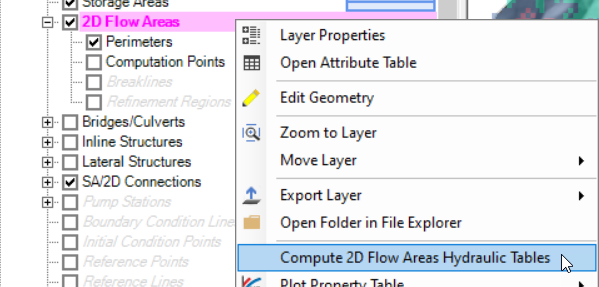
- Finally, compute the hydraulic tables for the mesh.
Connect 2D Flow Area to Cross Section with Existing Lateral Structures
- Close RAS Mapper and open the Geometry Editor
- Open the new Geometry - "Existing – 2D Levee Area"
- Using the Lateral Structure Editor, connect all the Lateral Structures to the new LockHaven 2D Flow Area. This includes 23100, 21200, 14800, and 11950.

- Notice that the plot displays the cell faces and the minimum cell elevation that the weir is connected to (you may have to switch the plot after hooking up the LS to LockHaven
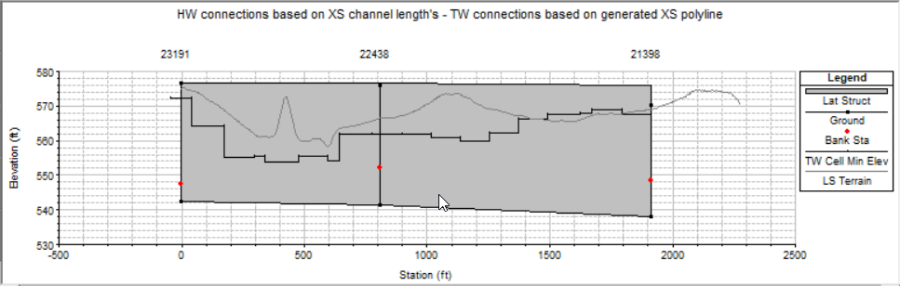
- Notice that the plot displays the cell faces and the minimum cell elevation that the weir is connected to (you may have to switch the plot after hooking up the LS to LockHaven
- Rename the SA/2D Area Conn labeled "SA191to190" to "LockhavenTo190" using the "Edit | Change Name" option in the Geometric Data Editor

- Using the SA/2D Area Conn. editor, connect the renamed connection to the the 2D Flow Area

- SAVE the Geometry Data. Then close the geometry editor.
Make a New Plan for the 2D Flow Area Geometry
- Open the Unsteady Flow Analysis window and open the existing 1D Plan "Existing Conditions 1D -1000 yr event"
- Choose NO when asked to save the current plan.

- Choose NO when asked to save the current plan.
- Make a new Plan file using the Save Plan As option from the File menu and call it "Existing 2D Levee – 1000yr. Give the Plan a relevant short ID, "Exist-2D-1000yr"
- Select the new 2D Geometry File for the new plan.

Perform Computations and Review Model Output
- Run the new 2D Plan. When the model has finished running, compare the 1D model to the 2D Model with the Profile Plot, Hydrograph plots, and RAS Mapper
As shown in below, there is very little differences in the profiles between the two plans. This was due to the fact that the same amount of flow went over the levees for both Plans. The tailwater elevations at each weir was very different between the 1D Storage Area model and the 2D Flow Area model. However, the tailwater elevations were not high enough to submerge the weir (levee), and therefore did not impact the computed flow over the levees.

The most upstream lateral structure (River Station 23100) had very different tailwater elevations. This is because the Tailwater elevation for the 2D Flow Area is reported the cells that are directly connected to the lateral structure, and the tailwater for the 1D model is the single storage area 192.
When water goes into the storage area, it immediately goes to the lowest point in the storage area, and then fills up as a level pool. When water goes into the 2D Flow Area it goes directly into the cells that are right at the edge of the levee and then routes. The overland from cell to cell based on the terrain and physics of the flow. For this specific model, the water surface in the cells ended up being much higher than the water surface of the 1D storage area. This could potentially create a difference in levee overtopping flow if the event were larger.
In general, it is believed that the 2D model lateral structure flows would be more accurate since they are computing the water surface on the tailwater side more accurately.

There is a Point Shape file loaded under the Features Layer called PointsOfInterest.shp that has three locations of interest. Turn on the layer and describe the differences in terms of time at which the streets got wet, peak stage, and time to peak using the table below What is the maximum velocity on the toe of the Lock Haven side of the levee?
| Location | Model Type | Arrival Time | Peak Stage (ft) | Time of Peak |
|---|---|---|---|---|
| Main & Mill Streets | 1D Storage Area | 03 Jan @ 06:05 | 566.67 | 03 Jan @ 15:30 |
| 2D Flow Area | 03 Jan @ 07:30 | 566.79 | 03 Jan @ 15:30 | |
| Church and Washington St | 1D Storage Area | 03Jan @ 06:40 | 566.67 | 03 Jan @ 15:30 |
| 2D Flow Area | 03Jan @ 07:40 | 566.79 | 03 Jan @ 15:30 | |
| Park and Prospect Streets | 1D Storage Area | 03Jan @ 04:55 | 566.67 | 03 Jan @ 15:30 |
| 2D Flow Area | 03Jan @ 06:35 | 566.79 | 03 Jan @ 15:30 |
The results in downtown Lock Haven end up being close to the same peak stage and time to peak. However, the arrival times are different as demonstrated in the tables above. This is due to the fact that the 1D/Storage Area model puts flow instantaneously into the lowest point of the storage area, and fills it as a level pool, whereas the 2D Flow Area actually routes the water. So, the 2D Flow Area model is much more accurate at arrival times and intermediate inundations as the event is unfolding.
You can visualize this by plotting/animating the flood depths to see how the flood arrives. Below the blue is the 2D model, clearly flooding an area not inundation in the 1D domain.

For the problem being analyzed the cell size is good. When animating the 2D results, the transitions are very smooth, and they follow the terrain accurately. The goal of this problem was to route water behind the levees to see the flow path, however, if we needed note detailed velocity results, increasing the cell size and terrain resolution would be required.
The model was set up with a 15 second time step for the 1D/Storage Area model. This turns out to be just fine for the 2D model with 100 X 100 ft grid sizes
To figure out an appropriate time step, on needs to look at the areas in the model where the velocity is the greatest. Then the Courant Number can be computed for the cell size. From the 2D Velocity Output, maximum velocities were found to be around 8.0 ft/s. Using the courant number equation to predict a time step (for the Diffusion Wave form of the equations), we get the following:

A time step of 15 seconds should be fine.
The terrain data is ok, but it is not super detailed. It is missing portions of the levee in a few places, and depending on the problem we are analyzing. Further, roads are missing which would affect arrival times but probably not max depths.
In general, it is difficult to know if the full shallow water equations will give a significantly different answer than the diffusion wave equations. The only true way to figure this out is to run the data set with both equation sets and compare the answers. The SWE will generally require a smaller time step for the same grid resolution and floodwave being modeled. This is due to the fact that the full equations have the acceleration terms, which are sensitive to changes in velocity with respect to distance and time. These terms generally require smaller time steps when there are significant changes in velocity with respect to distance and time.
To test this out, we ran the model with both equation sets. The following are plots of both results from key locations around the levee and inside the levee system.
This plot is from the Lateral Structure at River Station 23100. The stages and flow are very nearly the same. There is a minor difference for the TW for the stage on the protected side of the levee. The flow going over the levee is nearly identical. The small difference in the tailwater at this location appears to have minimal effect downstream in the town of Lock Haven.

This next plot is a Plot of Water surface elevation vs time in the middle of downtown Lock Haven.

In addition to these two plots the inundation maps were compared and they were basically identical. So for this data set and event being modeled, the Diffusion Wave method is giving the same answers as the Full Saint Venant equations.
This result may not be true for all events being modeled. So in general you will want to test this for a range of events, most the higher extreme events.
Bonus - Levee Breaching
As time allows...
- Save the Plan File as a new Plan, using the SAVE AS option.
- Add a levee breach into the Lateral Structure at River Station 23100.
- Add in the breach with the following information, using the "Levee (Lateral Structure) Breach" option under the Unsteady Flow Analysis Options menu

- Run the plan
Comparing the hydrographs for that Levee?
The volume of water going into Lock Haven for the two plans can be determined by looking at the Lateral Structure Hydrographs, specifically the “Flow Leaving” hydrograph, which represents the total flow going over and through the lateral structure (This includes the breach flow).
For the with and without breaching plans the volume of water that went into Lock Haven can be computed by adding the total flow leaving from the lateral structures at River Stations 23100 and 21200.

Total Volumes or LS 23100:
Without Breaching = 8,816 ac-ft
With Breaching = 30,511 ac-ft
Shown below the inundated area for the with breach (shown in Red) and the without breach (shown in blue). While the inundated area is not much greater, the depth is much greater. The final water surface elevations were the following:
Levee Overtopping Only = 566.8 ft.
With Breaching = 573.1 ft.

From the Detailed Output Table for the Lateral Structure at River station 23100:
Bottom Elevation = 566 ft
Breach Bottom Width = 700 ft