Download PDF
Download page Creating a Simple 2D Model.
Creating a Simple 2D Model
Data Files
You will be working with a section of the Bald Eagle Creek river near Lock Haven, PA. Data files for this tutorial are provided in the zip file.

Objective
In this workshop, you will learn how to create a simple 2D model with HEC-RAS of the main channel and floodplain area. This workshop will require you to use multiple terrain datasets to form one terrain model, develop a 2D mesh, provide inflow hydrograph information, downstream boundary conditions, and perform model runs.
Background
You will be working on Bald Eagle Creek near Lock Haven, PA. Flow hydrographs will be used to simulate flows from Joseph Sayer's Dam downstream to the town of Lock Haven and the confluence with the West Brach Susquehanna River. Inflows will also be specified for local tributaries on Marsh Creek, Beech Creek, and Fishing Creek. A Normal Depth Boundary Condition will be used.
Terrain Model Preparation
This part of the workshop will guide you through the process of importing terrain data. The terrain data will be used as the basis for the mesh used for 2D hydraulic computations.
- Start HEC-RAS.
- Start a NEW project using File | New Project… Go to the workshop directory for this workshop ("Creating a Simple 2D Model") and then providing a Title and File Name. Press OK to save it.
- Launch RAS Mapper
 .
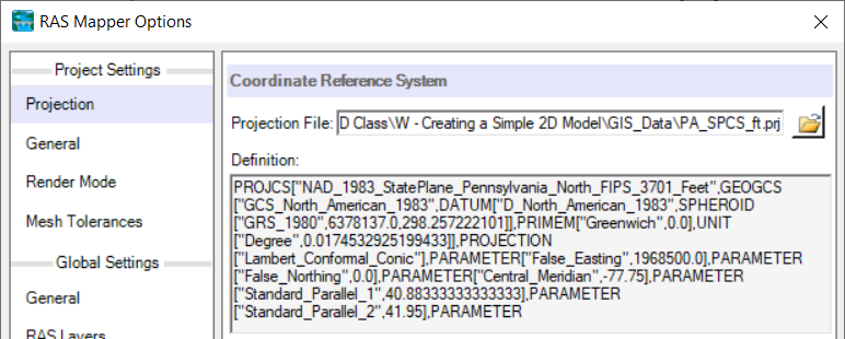
. - Select Project | Set Projection. Select the Folder button at the top left and navigate to the "PA_SPCS_ft.prj" provided in the "GIS_Data" folder. Select and Open this file. This sets the coordinate system for all the data you will view in RAS. The press the OK button to close the window.
- Import terrain data for use in RAS by selecting the Project | Create New RAS Terrain menu item.
- Click the Add Files
 button and navigate to the "Terrain" folder. Select the "BEC_10ft.tif" and "DEM.tif" files, then press the Open button at the bottom. The "BEC_10ft.tif" file contains gridded data at 10ft postings for the channel created from a TIN and the "DEM.tif" is a DEM (lower resolution) downloaded from the USGS for the remainder of the floodplain.
 - Use the New Terrain Layer dialog to order the files for import. Note that the "most important" layer should be on the top of the list and will get the highest priority when creating the Terrain Layer.
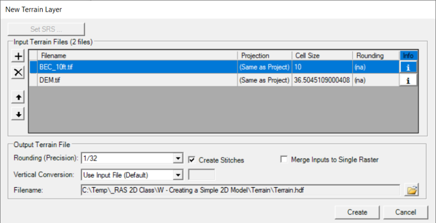
- Press the Create button.As the Terrain is created, a computation window will inform you of progress.
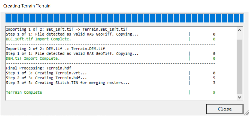
- When the terrain process is finished, select Close on the processing window, this will close both windows. Turn on the Terrain Layer.
- Right-click on the Terrain Layer and choose Zoom to Layer (if necessary to see the terrain).
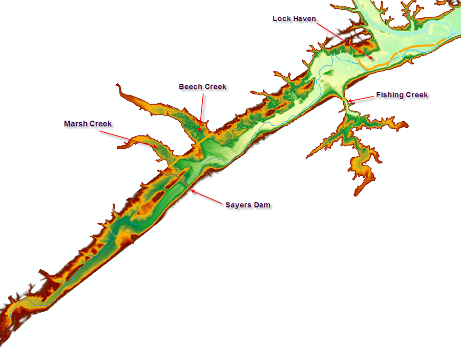
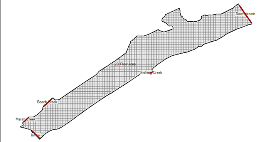
Below is what the terrain should look like. Also shown are all the boundary condition locations for this workshop.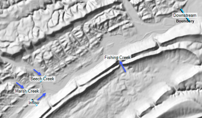
Note the location of Sayer's Dam (labeled Inflow) and tributaries, shown in the background image above. You will be creating a 2D Model below the Dam with tributary inflows.
Create the 2D Flow Area
The 2D Flow Area will go from just downstream of the Dam to the confluence (labeled Downstream Boundary) with West Branch Susquehanna River and will include a portion of Marsh Creek, Beech Creek, and Fishing Creek tributaries.
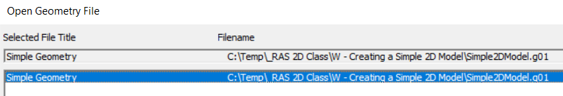
- Right-click on the Geometries group and choose Create New Geometry. Enter "Simple Geometry" for the name. Press OK to create the geometry layer.
- Right-click the new Geometry Layer and select Edit Geometry.
- Select the 2D Flow Areas Perimeter layer. Draw the perimeter using the Add New Feature
 tool.
tool.The polygon defining the 2D Mesh should capture the entire area of interest making sure that the polygon goes out to high ground. The high ground will ensure a “no flow” boundary (except at the inflow and outflow locations). However, the bigger your polygon the more cells you will have, the longer the computational run time, so sticking to the area of interest is important! If there are linear features in the land surface we want to make sure those are captured in the mesh (don’t worry about it for this workshop, we’ll do that in future workshops). Also, because of RAS quirks in mesh generation, making the polygon “smooth” will help with mesh generation, and reduce any problems in creating cells along the polygon boundary.
Also, since the water surface at the downstream boundary condition is unknown, in general we would want to go far enough downstream, such that when we apply a boundary condition like normal depth, that boundary condition does not have a significant effect on the water surfaces in our study area.
- Enter a name, when finished.

- In the Edit 2D Area Properties that come up, Enter 500 for the DX and DY Point Spacing.
- Click on the Generate Computation Points button.
- Change the Default Manning's n Value to 0.04.
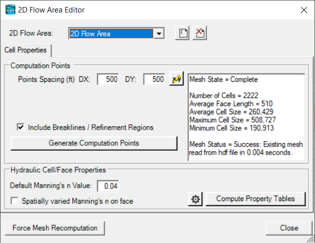
- Close the Editor.
- Turn on the Computation Points.
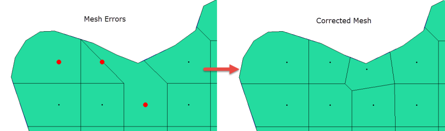
- Inspect the edge of the 2D Flow Area Mesh for any mistakes in the boundary. Make sure each cell has only one point in it. Turn off all background layers to more easily inspect the mesh. (Mesh problems should show up with cell points colored red.) To fix errors in the mesh, use the Editing Tools to Add, Delete, or Move points.
- Stop Editing to Save the Geometry!
Flow Data Connections
After creating the 2D Flow Area computation mesh, add all of the locations for flow boundary conditions.
RAS Mapper
- Start Editing in RAS Mapper.
- Select the Boundary Condition Lines layer.
- Create boundary conditions, left to right when looking downstream at each of the boundary locations shown below. Enter a name for each (Inflow, Beech Creek, Marsh Creek, Fishing Creek and Downstream).
Boundary Conditions must be drawn outside of the perimeter of the mesh!
Geometric Editor
- Close RAS Mapper.
- Open the Geometric Schematic and Open the new Geometry ("Simple Geometry").
- Verify the Geometry came in correctly. If not, fix it.
- Close the Geometric Editor.
Unsteady Flow Editor
- Open the Unsteady Flow Data editor and enter boundary condition information.
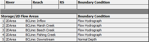
- Use Normal Depth with Slope = 0.001 for the downstream boundary condition.
- Use the "Simple2DModel_Flows.dss" file to define the Flow Hydrograph for the upstream boundary and tributaries. You will need to click the Add DSS File
 button to add the DSS file prior to picking a path.
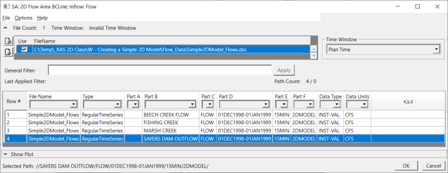
The hydrograph for the inflow is named "Sayers Dam Outflow". The other DSS records are named the same as the boundary condition.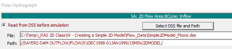
- Specify the "EG Slope for distributing flow along BC line" as 0.001. (This is located at the bottom right on the Flow Hydrograph window.) This must be done for all of the flow hydrographs attached to the 2D Flow Area.
- Repeat previous 2 steps for all inflow locations.
- Save the Unsteady Flow data when complete (call it "Flows").
Plan and Simulation
- Open the Unsteady Flow Analysis window, Save a Plan, and enter all of the necessary information to make a run.
- Set up the time window:
Start Date: 02JAN1999
Start Time: 0000
End Date: 06JAN1999
End Time: 0000 - Turn on the Geometry Preprocessor and Unsteady Flow Simulation programs.
- Specify a Time step
Deciding on the proper time step for the 2D Simulation is similar to figuring out what time step to use for an unsteady-flow simulation in a 1D model. So, the question you should ask is “if my cross sections are spaced X feet apart (or in 2D my cell size is X feet), and my flood wave velocity is so fast, then to satisfy the Courant condition, my time step should be thisbig” (time step <= spacing/velocity).
For a 500ft grid-cell spacing and an estimated flood wave velocity of 10 ft/s, then a time step of 100s is appropriate. Adopting a time step of 1min would certainly be appropriate, while a time step of 2min would probably work out just fine and will most likely reduce the simulation time. If using the Diffusion Wave form of the unsteady-flow equations, satisfying the Courant condition of C<= 1.0 is not nearly so necessary as when using the full shallow water equations. In general, the Diffusion Wave equations are more stable.
For the 500 ft grid cell size, we selected a 1 minute time step to use for the initial model.
- Save a plan by the name of the grid cell size and time step selected ("Initial Run").
- Run the simulation (press the Compute button).
To create hydraulic tables for the 2D Computational Mesh requires a Terrain model; therefore, you should have associated the Terrain with the Geometry. In this case, since only one Terrain was specified, RAS figured out which Terrain to use. However, good practice is to NOT rely on RAS to make good decisions for you!
- Go to the Options | Calculation Options and Tolerances and set the 2D Flow Option for the Initial Conditions Time (and Ramp Up Fraction).
- Simulate various timesteps.
The Initial Conditions time allows the 2D model to put water everywhere in the model where base flow should exist. This is not going to be just based on a travel time in the river, but rather how long it takes to fill areas that should be wet. After running an initial simulation, you will find when water has filled the low-flow portion of the river.
For the main Bald Eagle Creek portion of the river, the initial flow is very low. You would need to put in a reasonable “minimum flow” to fill up the channel. The initial flow from the inflow hydrograph is very, very low and, therefore, takes a very long time to fill the channel. Increasing the minimum flow to 400cfs, requires a warmup of about 20 hours to get the river stages to a reasonable elevation.
The base flow and rising portion of the hydrograph will fill the channel. This may leading to incorrect flood volumes, peaks, and timing.
One way to help speed up the simulation time is to make your first run and create a Restart file at the end of the warm up time period. This can be done from the Options | Output Options menu item on the Unsteady Flow Simulation window. Set a Restart file to be created at the beginning of the simulation. This creates a file “Simple2DModel.p01.DDMMMYYY hhmm.rst” and can be used in the unsteady flow file for the initial conditions.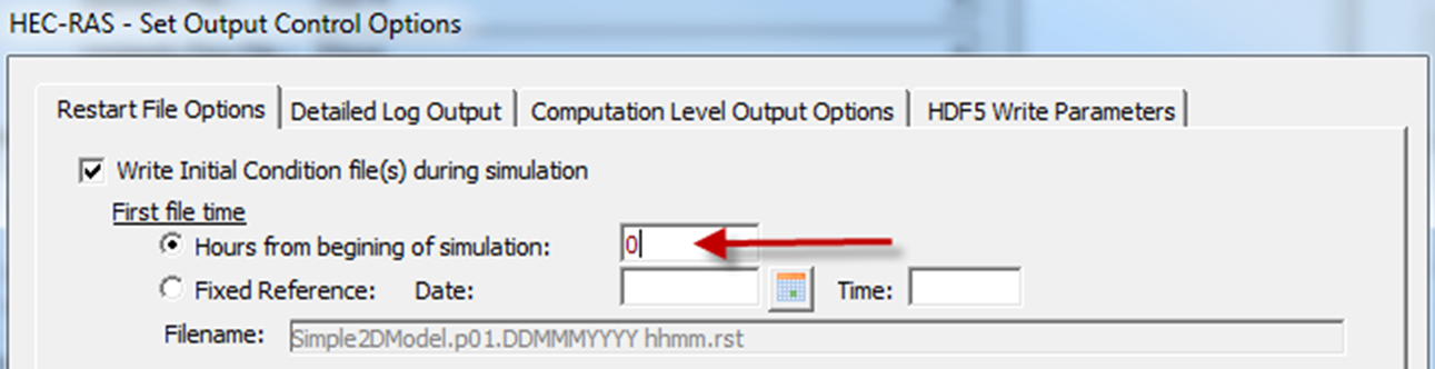
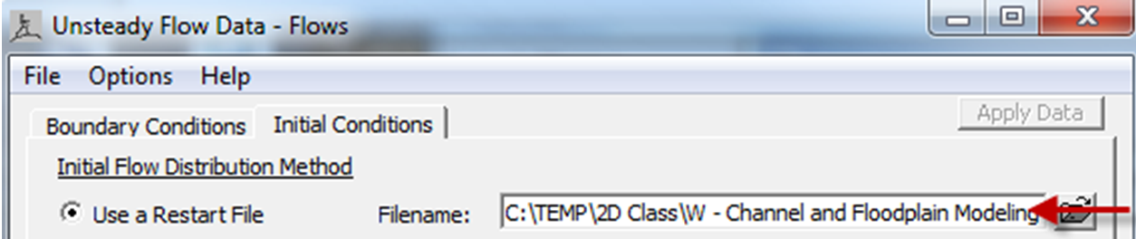
Next, go to the Unsteady Flow file, select the Initial Conditions tab and select the Use a Restart File option. You will then select the restart file to use.
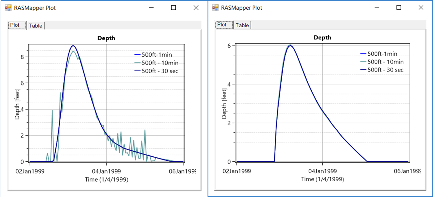
Several different time steps were used for the simulation (1min, 10min, and 30 seconds). The Water Surface Time Series option was used to plot the water surface at various grid cells, but specifically at the Walmart. It was noted that there is very little difference in the water surface for the 1min, 10min, and 30 seconds time step down near the town of Lock Haven (for the 10min time step <0.1ft difference is observed). However, the hydrographs below demonstrates the instability that will be produced by selecting an improperly large time step (the hydrograph on the left is up below the dam, the other is downstream near the town). See the jagged (unstable model) plot for the large time step compared with the appropriate time step, below.