Download PDF
Download page Dam Breach Analysis with 2D Areas.
Dam Breach Analysis with 2D Areas
Data Files
You will be working with a section of the Bald Eagle Creek river near Lock Haven, PA. Data files for this tutorial are provided in the zip file.

Objective
In this workshop we will be performing a dam breach analysis to determine the consequences of a failure of Sayers Dam by inputting design inflows for the reservoir and setting the Sayers Dam to breach. This workshop will guide students on using HEC-RAS to:
- Create a new dam breach model using 1D and 2D elements
- Connect 1D and 2D elements using SA/2D Connections
- Set a SA/2D Connection to breach
- Interpret the results of a dam breach simulation
Background
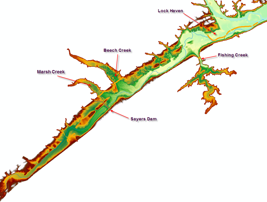
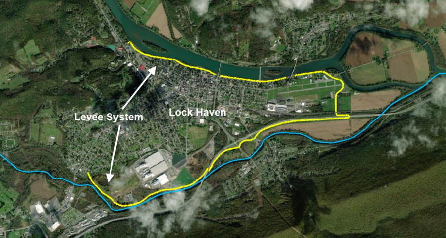
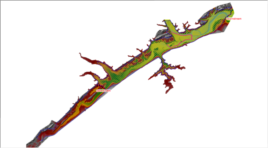
The town of Lock Haven is situated on the north bank of Bald Eagle Creek in central Pennsylvania. Lock Haven sits behind a levee system that was designed to provide protection for a 500-year (0.2% Chance) event. Sayers Dam, a flood control project on Bald Eagle Creek, is approximately 15 miles upstream of Lock Haven. See the figures below to become acquainted with the domain.
Create the HEC-RAS Project
- Create a new HEC-RAS project in the "2D Dam Breach" directory. Name it "BaldEagleCreekDamBreach"
- Open RAS Mapper
- Set the projection from a projection in the "GIS_Data" directory
- Add the Existing RAS Terrain ("Terrain.hdf")
Create the Geometry in RAS Mapper
- Add a New Geometry
- Start Editing the Geometry
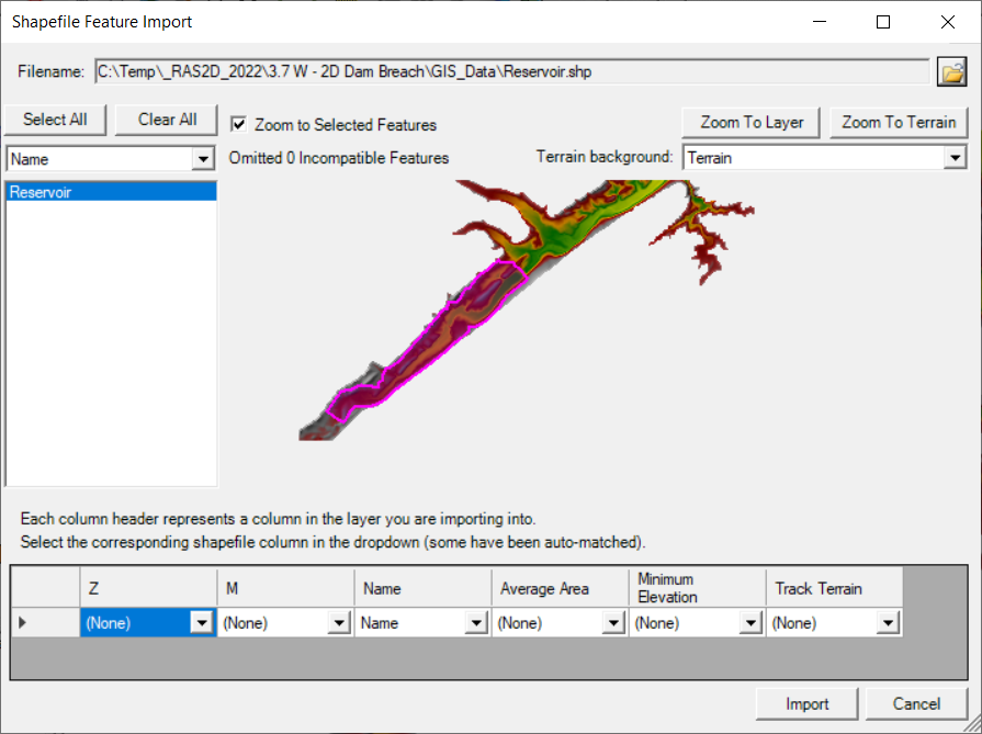
- Create the Reservoir behind Sayers Dam
- Select the Storage Areas layer
- Import the "Reservoir" shapefile (GIS_Data folder)
- Create the 2D Flow Area
- Expand the 2D Flow Areas layer
- Select the Perimeters layer
Import the "Downstream Area" shapefile (GIS_Data folder)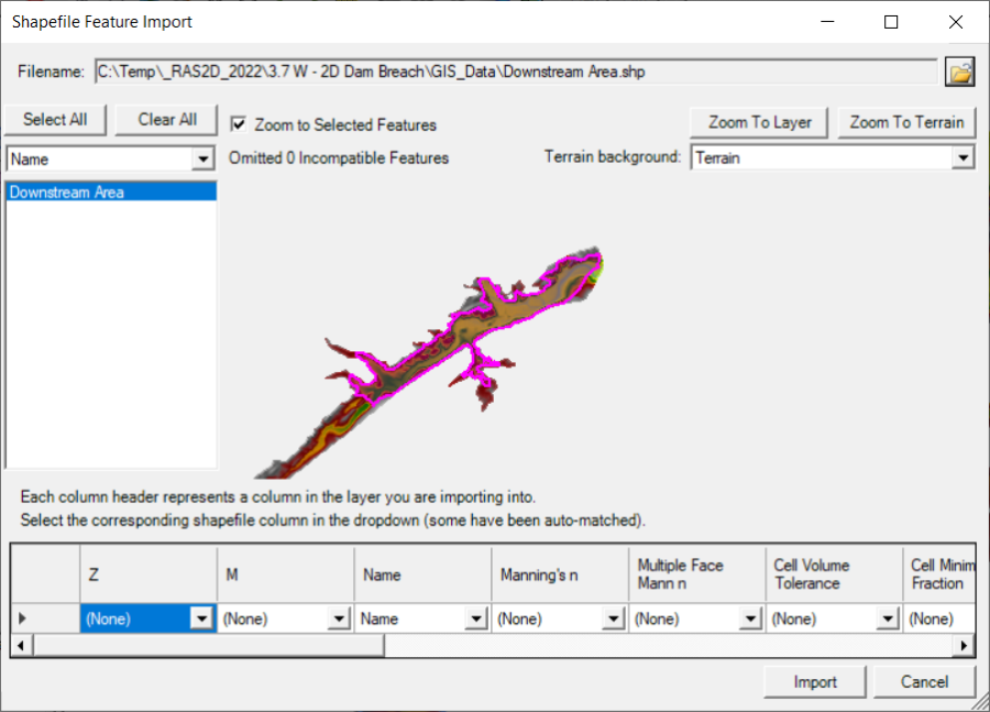
- Right-click on the perimeter and choose Edit 2D Area Properties.
- Set the cell size to 500ft
- Set the Manning's n value to 0.04.
- Generate computation points for the 2D Flow Area
- Inspect the mesh for bad cells
At this point you should have a Storage Area and a Mesh, as shown below.
- Create Breaklines along the levees
- Import the Levee shapefile for the upper, middle, and lower levee to the Breaklines layer.

- Right-click on the Breaklines layer and choose Enforce All Breaklines to modify the mesh.
The mesh should look similar to the figure below.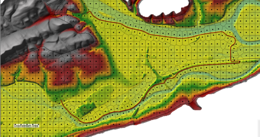
- Import the Levee shapefile for the upper, middle, and lower levee to the Breaklines layer.
- Create the Dam
- Zoom to the Dam location
- Select the SA/2D Connections layer
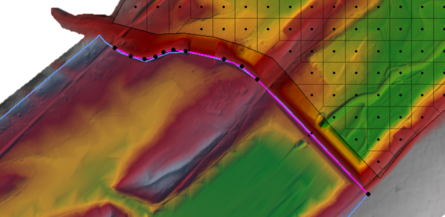
- Draw the structure along the top of the dam, left to right when looking downstream. (We will override the weir elevations later)
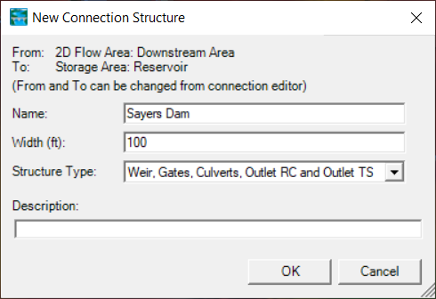
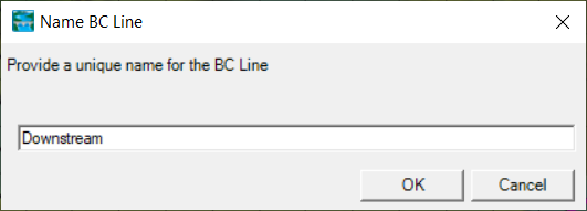
- Provide a Name
- Create the Downstream Boundary
- Zoom to the lower end of the model
- Select the Boundary Condition Lines Layer.
- Draw the Downstream Boundary line and provide a Name
- Stop Editing, saving the edits.
- Close RAS Mapper
Complete the Reservoir
- Open the Geometric Data Editor
- Open the Geometry
- Edit the Storage Area Note that there are already data provided. These E-V data were extracted from the terrain model, but we need to replace with more accurate data.
- Enter the Elevation-Volume Relationship – this data is in the "BaldEagleDamBreachWorkshopData" Excel spreadsheet.

Complete the Dam Data (Weir Profile and Gates)
- Edit the SA/2D Area Connection
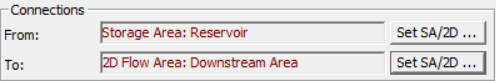
- Verify the From and To connection
- Replace the Weir/Embankment profile from the terrain (see below)
- The top of dam is 683ft, top of spillway is 657ft and the auxiliary spillway is 600ft wide. You will need to match the weir width with the centerline length. The final dimensions are shown below.(The length will vary based on how you drew the dam.)
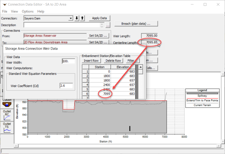
- The top of dam is 683ft, top of spillway is 657ft and the auxiliary spillway is 600ft wide. You will need to match the weir width with the centerline length. The final dimensions are shown below.(The length will vary based on how you drew the dam.)
- Add Gates using the information specified below.
- Gate information is provided below. Two gates (that line up with the river) that are 15ft high and 7ft wide with an invert at 590ft.
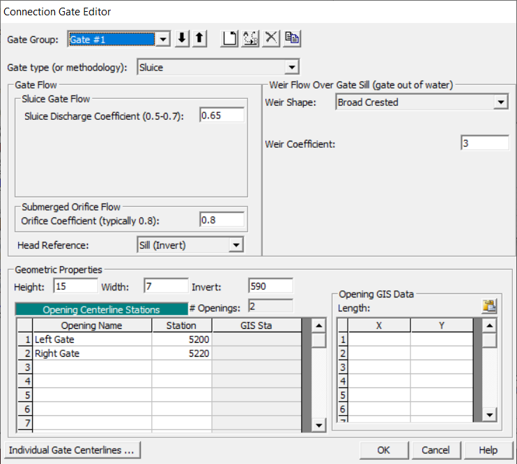
- Gate information is provided below. Two gates (that line up with the river) that are 15ft high and 7ft wide with an invert at 590ft.
- Save the Geometry
Enter Flow Data and Boundary Conditions
- Open the Unsteady Flow Data editor
- Use Normal Depth for the Downstream Boundary with S=0.0003.
- Use a Flow Hydrograph for inflow into the Reservoir.
- Click Add SA/2D Flow Area button
- Select the Reservoir
- Add a Lateral Inflow Hydrograph to the Reservoir
- Increase the number of points in the table to 200 using the No. Ordinates button

- Copy and paste the flow hydrograph from the Excel sheet
- Set the Gate Openings
- For Sayers Dam, set the boundary type to Time Series of Gate Opening.

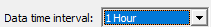
- Change the Time Interval to 1 hour
- Change the number of ordinates to 200
- Set the opening to 2ft.
- For Sayers Dam, set the boundary type to Time Series of Gate Opening.
- Set the Initial Conditions for the Reservoir Pool
- Click on the Initial Conditions tab
- Set the Reservoir to 630 ft.
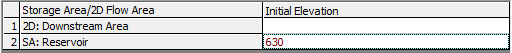
- Leave the 2D Flow Area blank. It will start dry.
- Save the Flow Data
Create a Plan with Breach and Simulate
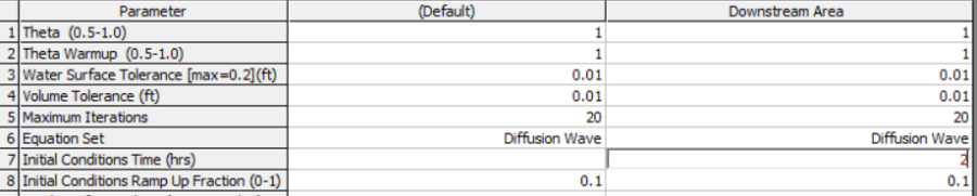
- Set up the plan with a 5-day simulation window
- Set the plan with a reasonable time step
- Set the Initial Conditions Time for the 2D area to 2 hrs
- Set up Breach Parameters as shown in the figure below

- Turn on Breach This Structure
- Save the Plan Data.
- Compute the results.
Review Results
After running the model, review the output and answer some questions.
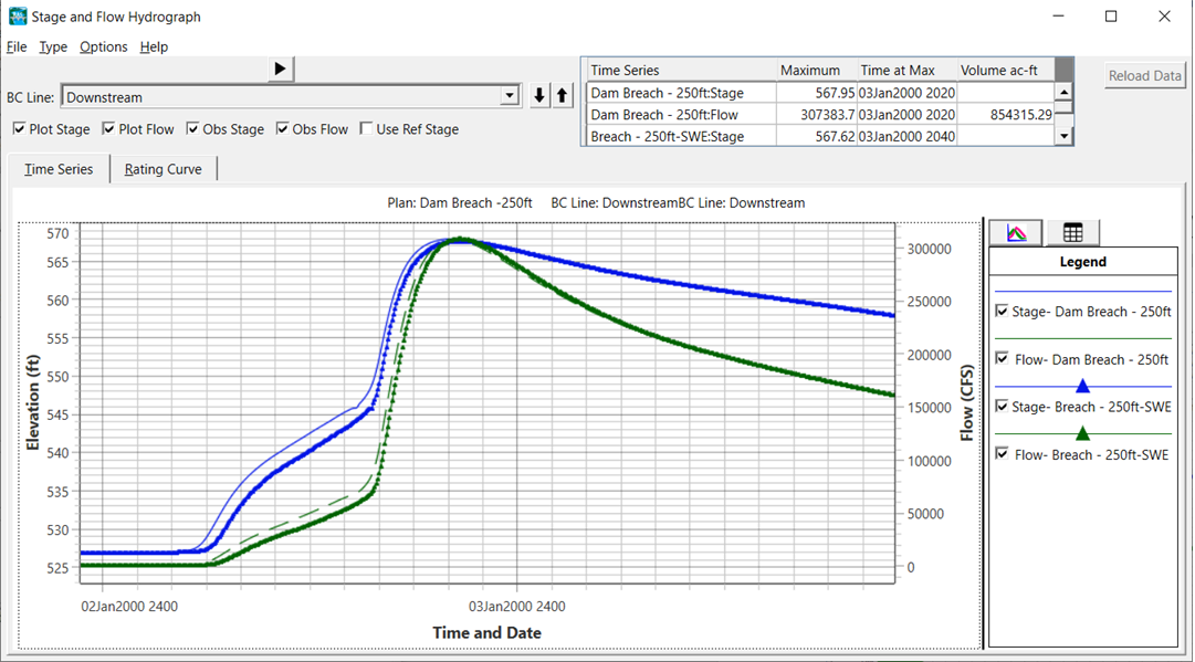
Based on the hydrograph plot for the 2D Connection, the Peak Outflow is ~516,000 cfs (~435,000 cfs is breach flow). The plot below shows the stage and flow hydrograph for the hydraulic structure around the time of the breach.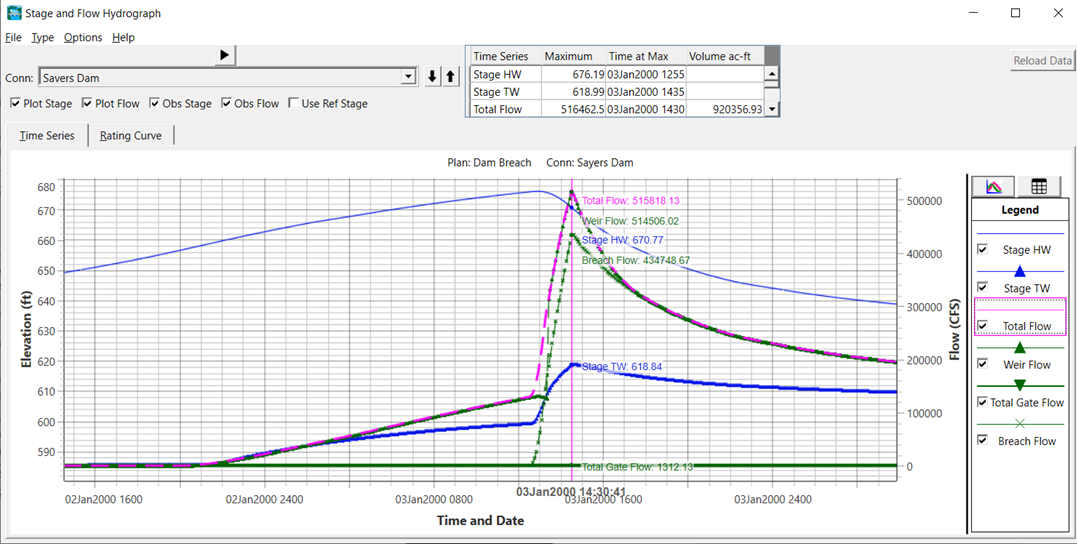
The flow hydrograph for the Downstream Boundary shows ~305,000 cfs.
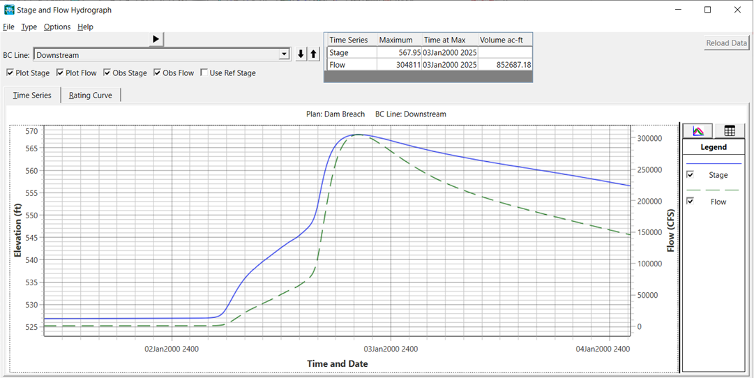
This flow is reasonable. Approximately, 200,000 cfs of peak flow was attenuated during the breach. The run time messages indicate a 0.02 percent volume error.
This, however, does not mean the results are accurate. There are many factors that we will need to investigate for model sensitivity that could affect accuracy.
- Accuracy of the hydrology
- Breach parameters (size and formation time)
- Terrain data
- Representation of the main channel, levees, roads, and high ground barriers
- Representation of levees, roads, and high ground barriers in the 2D mesh
- Manning’s n values
- Downstream boundary condition
Lateral inflows and local flow (which we didn’t use)
This initial solution was run with a 20s time step. Given a 500ft cell size and velocities of up to 25 ft/s, a time step of 20s satisfies a courant condition of 1.0.
We would need to test the model by running a various time steps and evaluating the impact on flow specific locations of interest to identify the impact. For instance, the levees are overwhelmed by the flood event and rapidly overtop. More accurate computation of flow would occur with a smaller time step.
No! Using a cell size of 500 ft does not accurately pick the details within the Lock Haven leveed area and the levee itself. However, this levee could be modeled with a separate hydraulic structure. The area inside the levee would also benefit from a smaller cell size, and additional break lines.
Bald Eagle Creek gets very constricted through the Lock Haven area. With a cell size of 500ft we only have 1 cell across the entire main channel. While HEC-RAS can route flow this way (due to the fact that the faces are like cross sections, and the cells have a detailed elevation volume curve), the flow is being computed more like 1D flow than 2D. Also, the contraction of the flow is very extreme at this location during high flows. This cell size may be too coarse to pick this up accurately.
The only true way to know if the cell size is appropriate is to run a smaller cell size and see if there is a significant difference in the results at various key locations in the model.
Change 2D Cell Size and Rerun
- Save the base Plan to a new plan ("Breach 250")
- In RAS Mapper, Save Geometry As and provide a new name ("Mesh 250")
- Start Editing the mesh,
- Change the cell size to 250ft, and Generate Computation Points with All Breaklines.
- Stop Editing
- Select the new Geometry for the Plan
- Select an appropriate time step
- Compute
- Review the following questions
Because we changed the mesh size, we should have also reduced the time step.
Total flow did not appear to change significantly. Any differences would most likely be due to the smaller cell size produces a higher tailwater elevation and submergence differences across the auxiliary spillway.
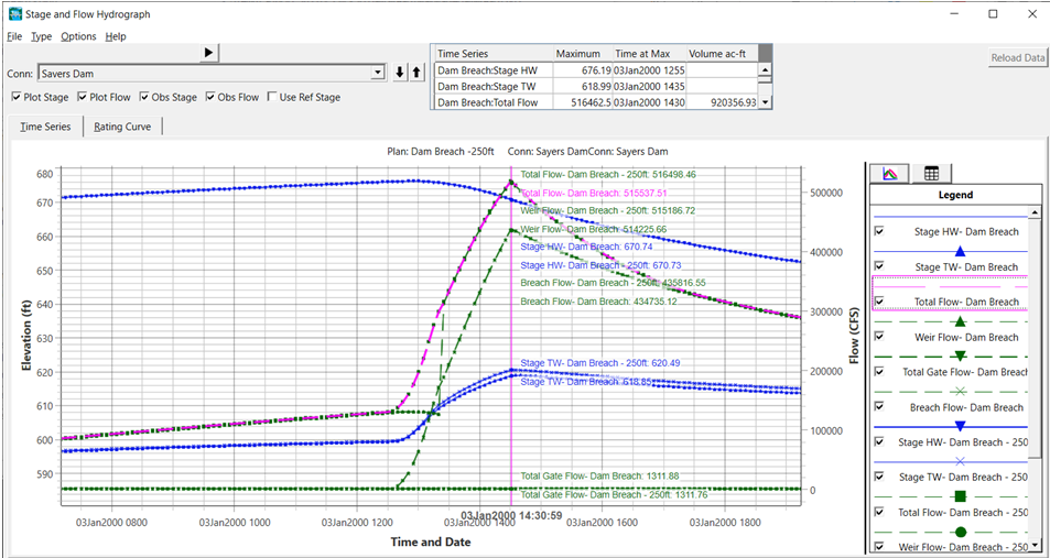
There is very little difference in the outflow.
Look at the Max Depth inundation, as well as different time steps during the event to answer this question. The 500 ft plan map was changed to red and put the 250ft plan is in blue on top.
You can see the larger cell sizes allow water to spread faster.
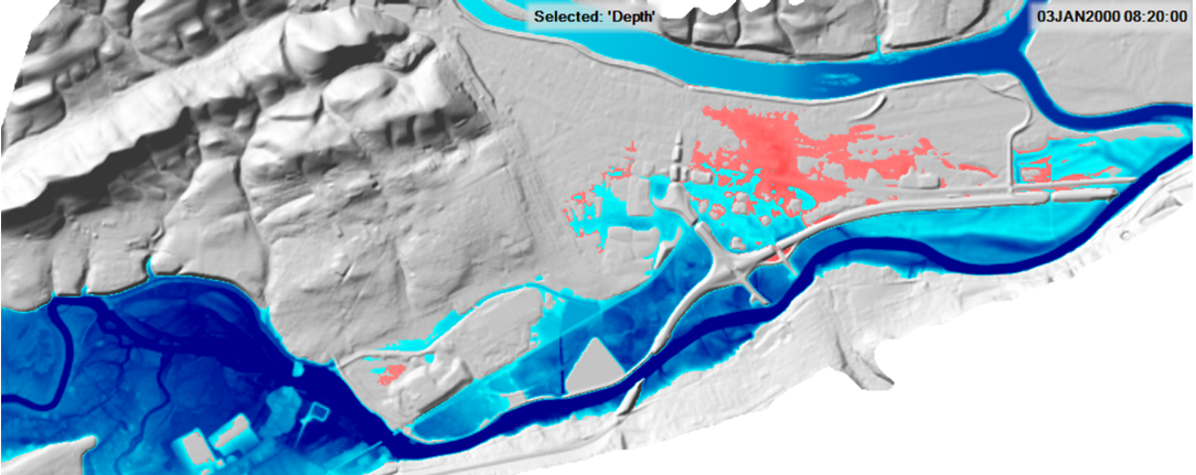
There was very little difference in the maximum inundation, which is easily seen with a time series plot of WSE.
Is it detailed enough with this cell size? If not, what are the options you could use to model the Lock Haven levee system more accurately than it is currently represented in this model?
Not really. While the 250ft cell size is better overall for this model, the levee is still not being modeled adequately. Some options to better model this system are discussed below.
- Model the whole system with a very small cell size, such as 5 to 10 ft grids. However, this would still require that the levee be accurately represented in the terrain model. This is not the case for this terrain data set, so this option would not work here. Also, this would generate a tremendous number of cells. A 10ft cell size would end up being 8 million cells for this same area. This would also require an extremely small time step, on the order of 1 second. This would not be feasible for this problem.
- The area inside the levee system could be modeled as a separate 2D Flow Area, with its own cell size, roughness, etc.. The main river and floodplain could also be a separate 2D Flow Area. Then the levee could be modeled with SA/2D Area Hydraulic Connections to represent the levee. This would allow for the analysis of levee overtopping and breaching at any location.
- For the single 2D Flow Area approach, because the terrain is not detailed enough, an interior hydraulic structure could be added on top of the aligned faces to represent the levee more accurately. By putting in a hydraulic structure, the user can enter station elevation data for the structure that may be more accurate than the terrain data. The flow over the hydraulic structure can be computed as 2D over flow, or it can be modeled as 1D weir flow (this is a user choice). Additionally the use of the interior hydraulic structure allows the user to evaluate levee breaches (when using the weir flow option!), which cannot be done without the hydraulic structure added in.
While the modeling of the levee would be much more accurate with an added hydraulic structures, the 250 ft cell size may still be too coarse for the extreme constriction of the flow that occurs due to the Lock Haven levee and the steep mountain side, as well as the extremely rapid rising water surface due to the Dam breach/PMF.
In general, for a rapidly rising event like a dam breach flood wave, the full Shallow Water Equations are more accurate. The dam breach will have very high velocities just downstream of the Dam, and the water surface elevations and velocities will be changing rapidly as the floodwave moves downstream from the dam.
However, the only way to really know the significance in the difference between running these two equation sets, is to run them both for the same exact model and flood event. In general, the SWE will require a smaller time step for the same cell size and flood event, over the Diffusion Wave equations. This is due to the added complexity of including the acceleration terms and their associated derivatives. The full equations are more difficult to solve in a stable manner, especially for a dam breach flood wave.
Running the 250 ft grid model with the DWE (~3min runtime) and the full SWE (~15min runtime) as two separate plans requires saving the plan, changing the equation set, and setting a reduced time step. In general, the SWE ended up with higher water surfaces upstream of and through the levee system, due to the inclusion of the acceleration terms in the equations. This is due to significant contractions and expansions of flow in this model in many locations, especially in the area of the levee system.
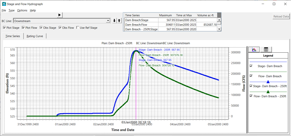
A hydrograph plot just upstream of the river’s constriction is shown below.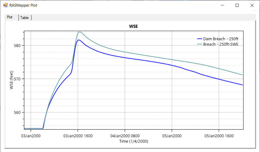
Another plot for the downsteam boundary shows peak stages are similar, however the DW solution has the floodwave arriving a bit sooner.