Download PDF
Download page Simplified 2D Bridge Modeling.
Simplified 2D Bridge Modeling
Data Files
Data files for this tutorial are provided in the zip file.

Objective
This workshop will help students learn how to use HEC-RAS to use the 1D bridge option inside a 2D flow area. The workshop will begin by developing a base geometry and plan that models a section of river with the shallow water equations (SWE) and then another geometry and plan will be developed with a 2D Connection structure that will operate in bridge mode to simulate a road crossing. These simulations will then be compared.
Background
The figure below shows the terrain and bridge crossing (flow west to east). The floodplain is highly constricted at the bridge which includes four rows of piers, these piers are marked by purple lines in the view below. The square piers have 4ft sides.
The flow event modeled does not overtop the bridge or hit the low chord.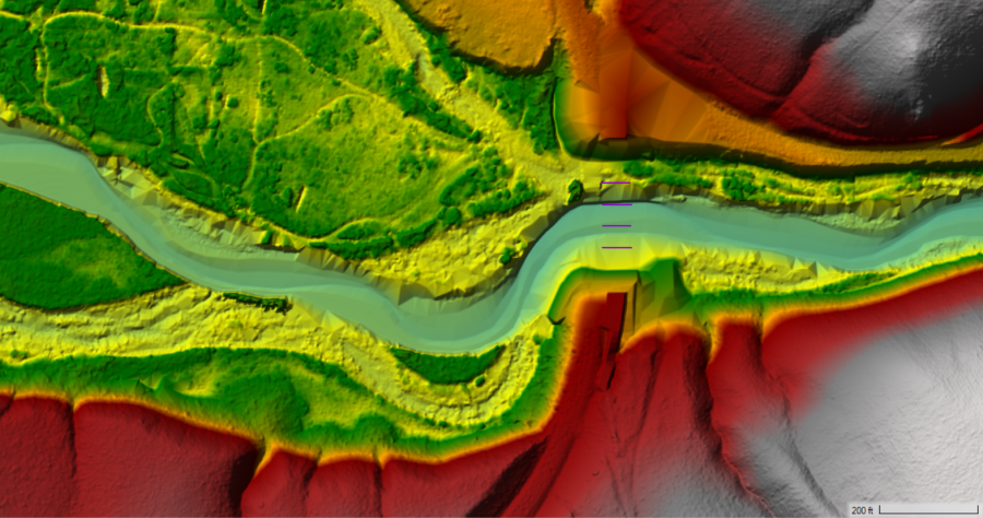
Create Initial Model Geometry
- Open HEC-RAS and start a new project
- Open RAS Mapper
- Set the projection ("GIS_Data" folder)
- Create a New Terrain ("Terrain" folder)
- Add a New Geometry.
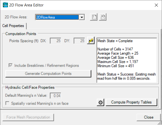
- Set up a coarse 2D Flow Area mesh for the entire study area.
- Try 25ft cells with a n value of 0.04.
- Set up boundary condition lines
- Inflow
- DS Boundary

- Stop Editing in RAS Mapper.
- Close RAS Mapper
- Open the Geometric Data editor.
- Open the initial Geometry
- Close the Geometric Data editor.
Enter Flow Data and Boundary Conditions
- Open the Unsteady Flow Data editor.
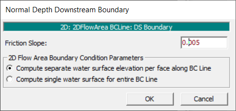
- Set the downstream boundary to use Normal Depth, s = 0.005
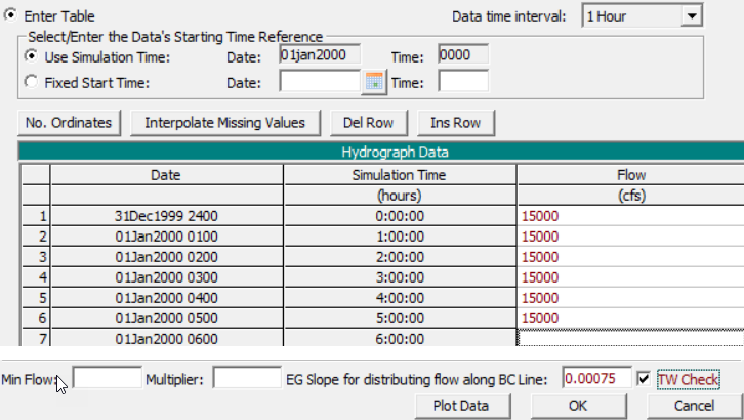
- Set the inflow to be a Flow Hydrograph Use a constant flow of 15,000 cfs. Set the EG Slope to 0.00075
- Save the flow data
Create a Plan and Simulate
- Open the Unsteady Flow Analysis window
- Set up the time window, time step, and mapping output interval.
- Set the Computation Options
- Set the Equation Set to SWE-ELM (original/faster) and the Initial Conditions Time
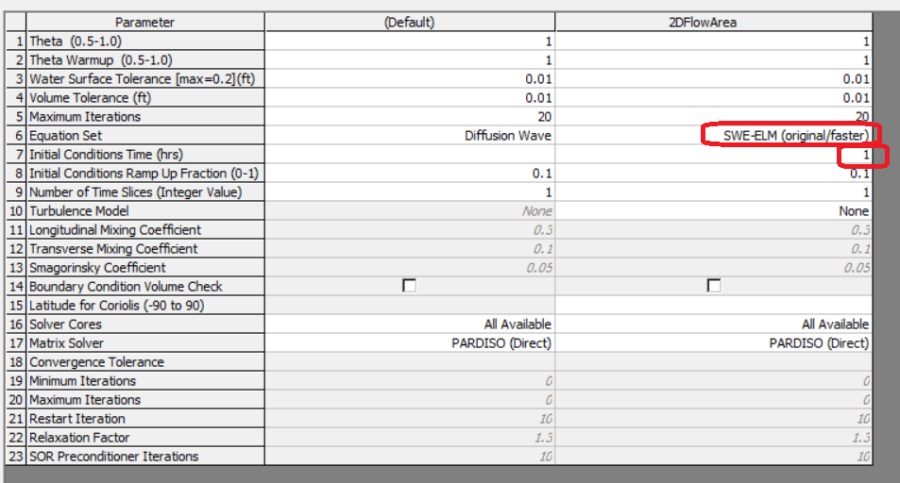
- Set the Equation Set to SWE-ELM (original/faster) and the Initial Conditions Time
- Save the plan data as Base Plan
- Compute
- Computation Time Step Check ensure solution is smooth and stable, pick a new time step and re-run if necessary.
Create new Geometry and Plan with 1D Bridge
- In RAS Mapper window use the "Save Geometry as …" menu option to copy the base geometry to start.
- Start editing and draw a centerline for the bridge deck and set the width to 40 ft. (draw from left to right looking downstream, which will be top to bottom in this case).
- Enforce the 2D cell spacing around the centerline as appropriate.
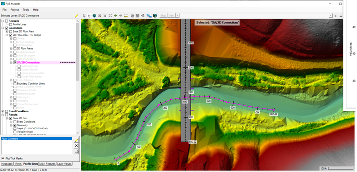
- Add the Pier Centerline shapefile (in the GIS Data folder)

- Turn on the stationing tick marks on the bridge centerline
- Note the bridge centerline stations where the piers cross it, you will need these stations when entering the pier data.
- Go the main Geometry Schematic and open the 2D Connection Data Editor.
- Ensure the structure type is modeled as Bridge (Internal to 2D Flow Area)
- Add a deck roadway that spans the full range width of the XSs with a flat top roadway at an elevation of 4615 ft and a low chord at 4607 ft.
- Set the upstream distance to 20ft.
- Select appropriate Weir Coefficient for this structure.
- Add 4 Piers that are 4ft wide at the stations you noted earlier where the centerline crossed the pier centerlines shapefile (spaced about 40ft apart).
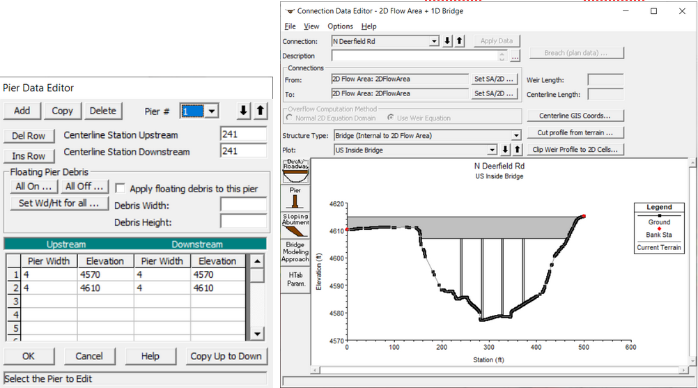
- Open the Bridge Modeling Approach and turn on the Momentum method and select an appropriate Cd coeficient for square nosed piers.
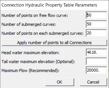
- Open the HTab parameters and limit the curves for this simulation.
- Open the "External and Internal Bridge Cross Section" dialog.

- Set the Manning's values for the 4 XS's for this structure to use a value or 0.04.
- Save geometry file.
- Save Plan As, to create another plan with this geometry.
- Compute
Compare Results
- Create a Profile Line for the river centerline. (turn on Plot Tick Marks to help find where the bridge is in the profile)
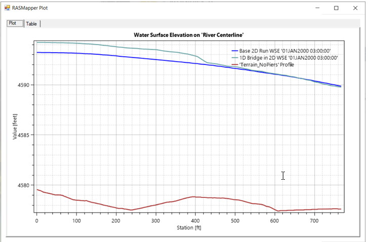
- Plot the WSE and compare the results.
The bridge causes about 1ft or rise in the water surface, that rise persists upstream to that US boundary of the study area. You would need to continue the model further upstream to see full extent of the impact of the bridge to the maximum profile.
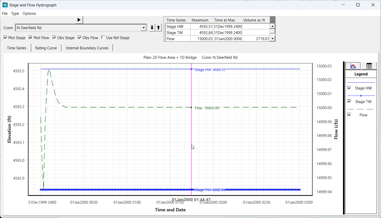
Plot the Stage and Flow Time series for the structure and see that the difference between the HW and TW is about 4593.5-4592.8 ~ 0.7 feet.
Click on the Internal Boundary Curves Tab and see the family of rating curves. The red circle is the solution. A red line has been added to show interpretation of the Tailwater to Headwater that was applied for the bridge loses.
