Expedited Debris Flow Tutorial

Expedited Debris Flow Modeling with HEC-RAS

Because of the emergency management implications of post-wildfire work, decision makers are often looking to understand their communities' risk very quickly.
There are several "expedited risk assessment" methods available and HEC-RAS is often considered a "detailed modeling approach".
But you can set up an expedited 2D HEC-RAS model very quickly, to provide actionable impact maps on emergency management time scales.

This workshop has two objectives:

Introduce you to the minimum required steps to build a debris flow model in HEC-RAS.
Demonstrate how to use HEC-RAS in an "expedited risk assessment" mode to bound the potential debris risk regions(starting with no data) in <an hour.
Expose modelers to the tools available to acquire the necessary data.

Therefore, this tutorial does not provide any starting files, only an online USGS post-fire hazard assessment link and an estimated max flow to simulate a data-sparse emergency management situation.

Note: The data and parameters used in this model are for educational purposes only. The models and parameters should not be used for engineering or scientific analyses. This workshop also reflects the quickest steps to get a result, not the best modeling practices.

Import Spatial and Terrain Data

Download Burn Area Shape Files

Go to the USGS Hazard site to download the burn area shapefile for this event.
https://landslides.usgs.gov/hazards/postfire_debrisflow/detail.php?objectid=289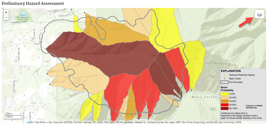

Press the layer button to explore the information provided for this fire.
(Note: You do not get to choose which of these you download, the download option provides all shape files).
Which sub-watershed d you think poses the most post-wildfire risk?

Scroll to the bottom of the page and right click on Shapefile (Shp).
Download the shapefiles associated with this event and unzip the folder.

2. Open Mapper and Create Project

Open HEC-RAS
Save Project As… and give the project a name like "First Debris Flow Workshop"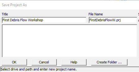

Open RASMapper. Select GIS Tools→RAS Mapper… or push the mapper button.
HEC-RAS indicates that the default unit system is US Customary when you create a new project.
Because we are starting with only the downloaded shape file and will adopt their projection), we need to use the unit system native to that projection…which is SI.

Switch the Unit System

Select "Options--> Unit System" nd select System Intentional (Metric System).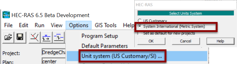

Note: This only sets the unit system, it does not convert the unit system. HEC-RAS not convert the projection units, so users must decide on the correct unit system before setting the projection or importing the terrain.

3. Get Projection

The first thing you need for a HEC-RAS model is a projection file.
But the shape files you just downloaded already come with one.
Therefore, you can just specify one of the *.prj files from these burn-area shape files as your projection.
In RASMapper select "Project→Set Projection…"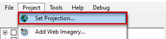

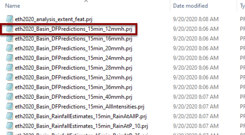
Press the Open button and navigate to the folder you just downloaded. This will show the projection files (*.prj associated with the burn area shape files. Select the projection:
Eth2020_Basin_DFPredictions_15min_12mmh.prj.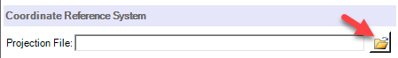

You can identify the unit system of the projection in the final line of the file, either in the *.prj file or in the report in the RS projection editor.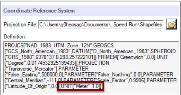

Press OK.

4. Import Burn Areas

You can drag shape files directly into RASMapper as Map Layers.
Open the folder that you downloaded the shape files into (and unzip them).
Then drag: the eth2020_Basin_DFPredictions_15min_12mmh.shp
shape file into the main RASMapper screen.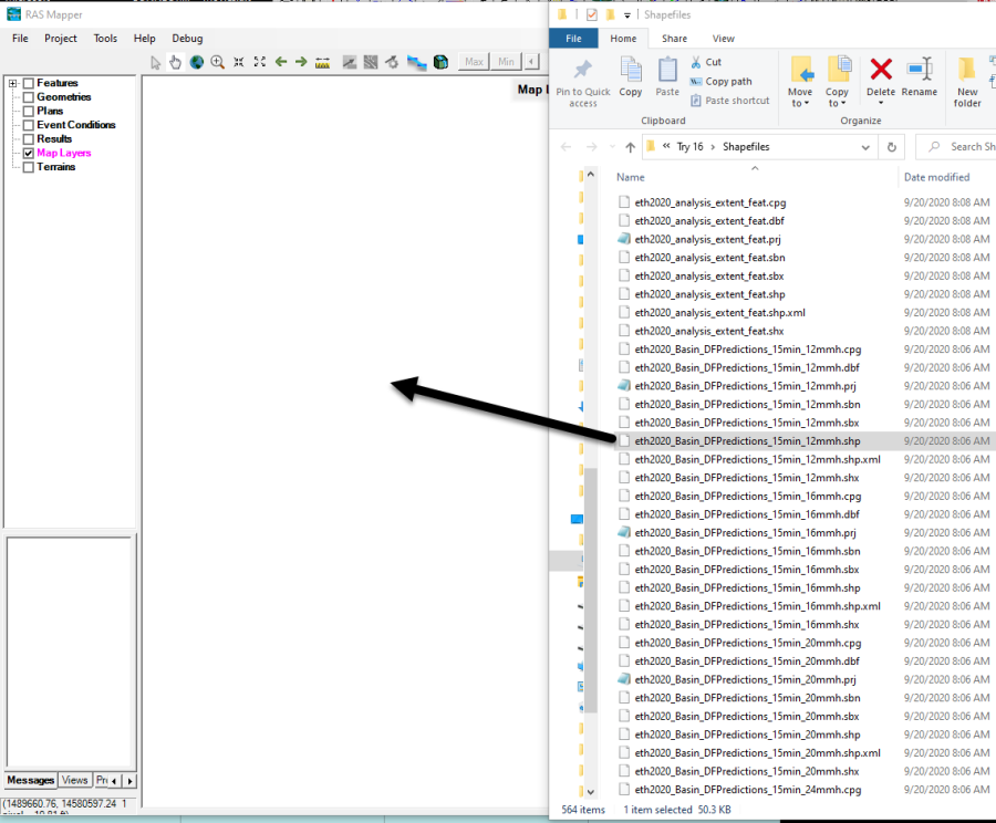

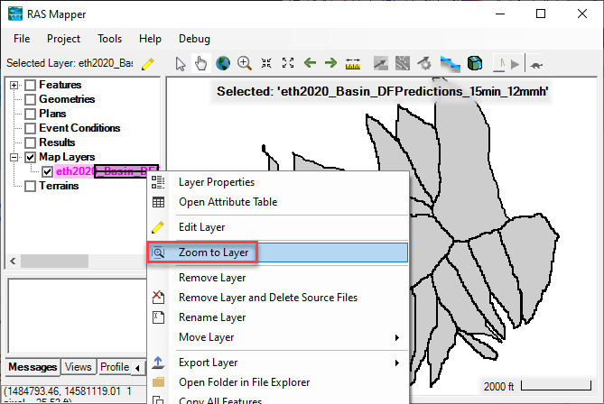
The urn area polygons will show up under Map Layers.
Right click on the shape and select Zoom to Layer

5. Turn Imagery On

Select "Project→Add Web Imagery" and choose Google Satellite.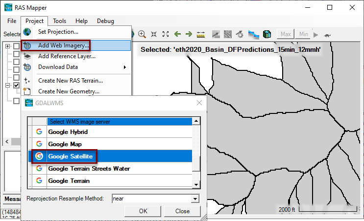

Turn on the Satellite imagery under the Map Layers menu.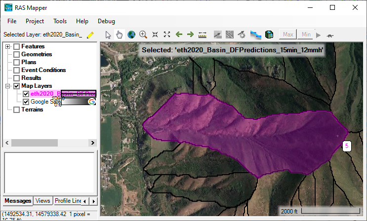

6. Download DEMs

The next thing you need is terrain data. RASMapper has access to the USGS terrain database.
Let's see what they have.
We will search by "Current View" so zoom out to include about a mile downstream of the burn watershed outlet.
Right-Click on the Terrains menu item in mapper. Select "Terrain → Download Terrain Data → USGS."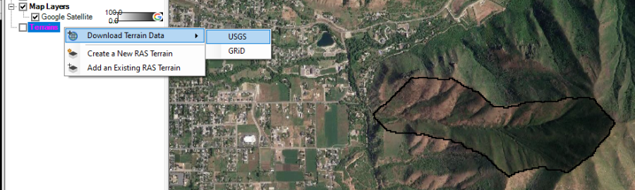

Leave the Import Extent Source as "Current View" and leave the Product Query Data Type as "Elevation Models" and press the Query Products button to see what DEMs the USGS has in this area.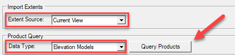

Note: If you have trouble with this query you can also query on the burn area shape file:

Use the temporary Map Layers (e.g. "USGS Products Available") to evaluate the spatial extent of these files. Then filter them to only include the 1m data. Press the Link to view metadata.

Does the 1m data look like it has the coverage we need to evaluate a debris flow runout about 2 km below this watershed? _______

Select both files, or if download times are long, you can just select the downstream DEM:
"USGS one meter x45y445 UT asatch-L5 2014"
HEC-RAS will create a Terrain subdirectory and will open it after these DEMs download

7. Create Terrain

Next you will have to "Create a Terrain" with the DEM's you selected. Right click on the Terrain menu item and elect Create a New RAS Terrain.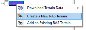

Press the "+" button to add DEMs to this terrain. Navigate to the USGS terrain folder and load the terrain(s) you downloaded. If you imported both, use the Up button to make the Wasatch DEM the top priority.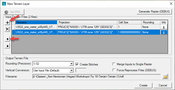

After you add the DEMs, you can Create the terrain.
Turn on the terrain you may have to turn off the imagery under Map Layers to see it.
If you right-click on the Terrain and select Image Display Properties , the Update Legend With View feature can be a helpful tool that rescales the colors if you zoom in on a part of the terrain.
Zoom in and see if you can identify the Alluvial Fan at the end of this watershed, where the high gradient basin transitions to the valley floor.

Create Geometry and Mesh

8. Create a Geometry File

Next you need a Geometry file. Right Click on Geometry Menu item and select Add New Geometry. Give it name like "10 m Mesh."

Note that the Terrain model will automatically be associated your new terrain.

9. Build Mesh

Click on the new Geometry layer and click on the pencil at the top of the Mapper Window (just above the navigation tree) to start editing. Expand the tree under the 2D Flow Areas group layer node and Click on Perimeters.
Draw a 2D Flow Area that starts near the downstream end of the burn area (just downstream of the final confluence (see figures below), includes part of the river corridor to the north, and extends at least a mile west.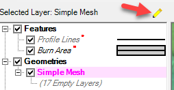

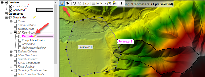
Double-Click to stop editing.
Right click on the Perimeter node and select Edit 2D Area Properties to generate your grid. Set a 10-m cell spacing and press the Generate Computation Points button.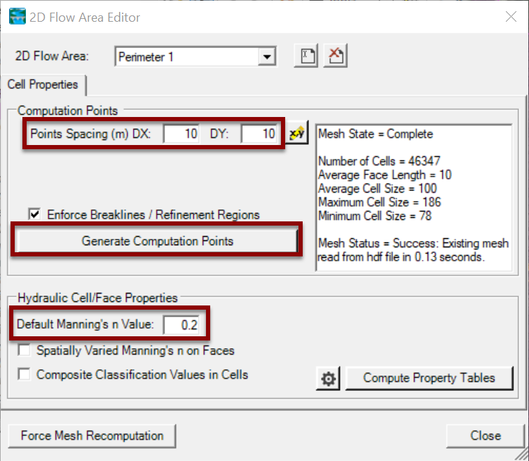

10. Define Upstream Boundary Condition

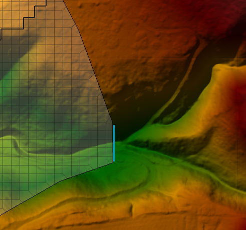
While you are still editing the Geometry, click on the Boundary Condition Lines menu item and press the Draw button again. Click to draw a boundary condition line along the upstream edge of the mesh where the channel enters it. (Note: the line must be outside the mesh and cannot intersect with it). Double click to finish the boundary condition.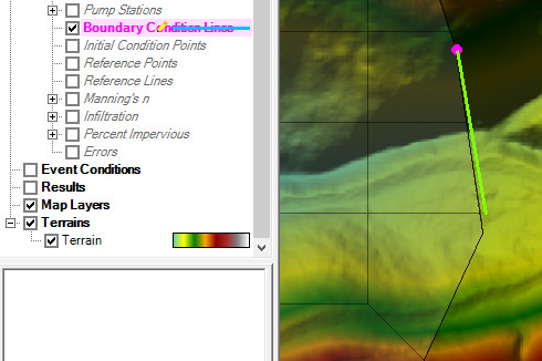

Press the Stop button or right click the geometry and select Stop Editing to finish editing.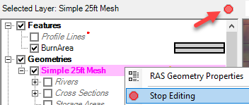

11. Open Geometry in the Geometry Editor

Because we made the geometry in mapper, we need to activate it in the Geometric Editor. From the main HEC-RAS menu, open the geometry editor by pressing the geometry button or selecting *Edit Geometric Data.*
In the Geometric Editor, Select *File Open* and open the geometry file you just made. hn save the Geomety.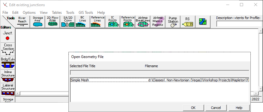

Create Flow and Plan Files (Without Debris)

12. Define Flow Data (without Debris)

Next, open the unsteady flow file to enter flow data. Press the Unsteady flow button or select "Edit→ Unsteady Flow Data..".
The boundary condition you defined should show up under Storage/2D Flow Areas. Click on that row under Boundary Condition. Then press the Flow Hydrograph button.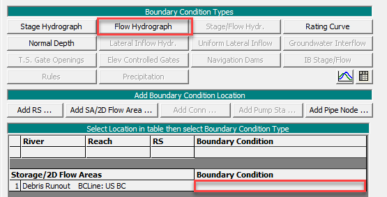

This will open the Hydrograph Editor (next page).
Click the radio button next to Enter Table.
We have an HEC-HMS model of this system, but we are trying to build a model with as little external data as possible, so we will use two hydrologic estimates to build this model.
Peak Flow = 9 cms
Event Duration ~1 hour
We will use those two data points to create a synthetic, triangular, hydrograph.
Choose the Fixed Start Time radio button and add a Fixed Start Time and Date.
Since this is a possible future event, it can be helpful to date it obviously in the future so it doesn't get confused with a historic event.
Set the flow editor to 1-minute intervals, so change the Data Time Interval to 1 Minute.
You will want to add rows to the editor to make sure you can cover a 6 hour run time so select the No. Ordinates button and set it to 400.

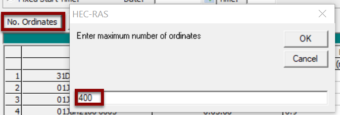
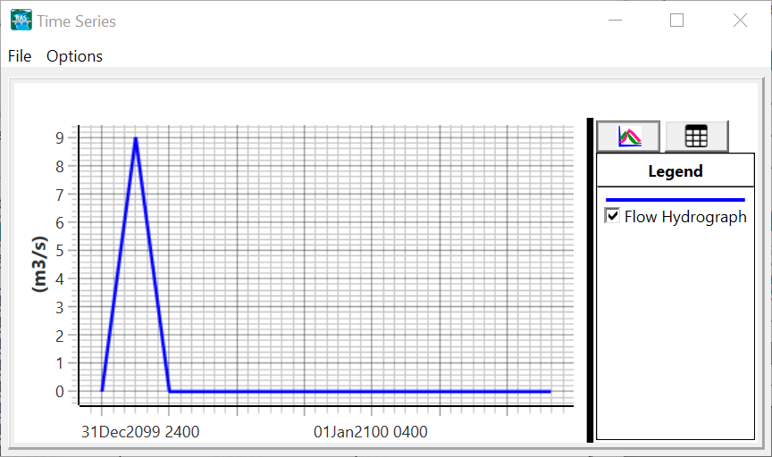
Next, you will define your synthetic, triangular, hydrograph with 4 points (and then interpolate between them).
Type in the following values a time 0, after half an hour, after an hour, and at the final time step:
0:00:00 = 0 cms (First Row)
0:30:00 = 9 cms
1:00:00 = 0 cms
6:39:00 = 0 cms (Last Row)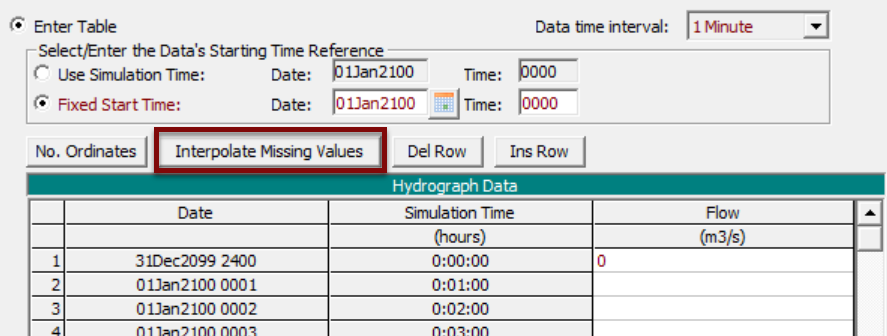

Then Press Interpolate Missing Values to fill out the missing values.
Press Plot Data to view your hydrograph.

The last required data field you must populate is the EG Slope for Distributing Flow along the BC line, required to distribute the upstream boundary condition across the upstream cells.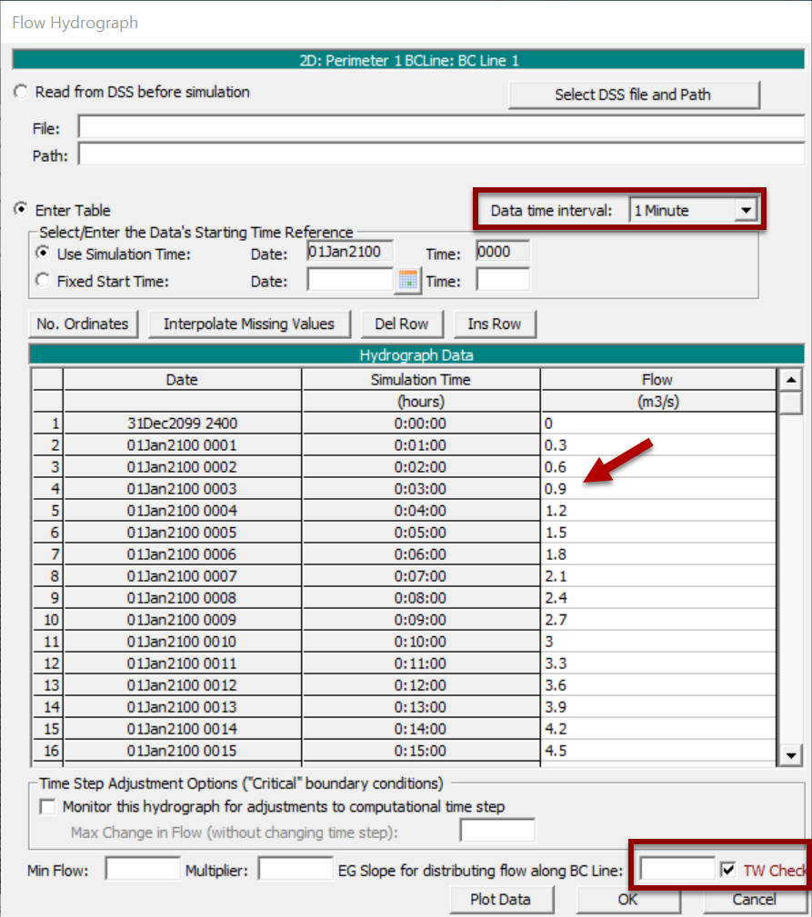

The easiest way to get this is to assume the Energy Grade slope will be close to the bed slope.
Then, you can use the Mapper measurement tool to measure the slope along the channel at your upstream boundary condition.
Select the "ruler" icon from the Mapper toolbar (see below) and draw a single line segment along the channel, perpendicular to the boundary condition line you just drew (see below).
When you double-click to finish the line, a dialogue box will appear and report the length of the line and the slope of the terrain under the line.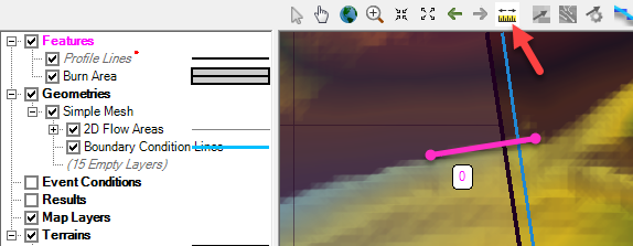

Save your flow file. Give it a name that indicates it does not include debris (e.g. "Clear Water" or "Newtonian".
Finally, click the check box called TW Check.
This helps boundary condition stability in steep models.

13. Create Newtonian Plan

In HEC-RAS, a "Plan" is a file that combines a geometry file and a flow file and add simulation parameters and instructions.
Open the Unsteady Simulation editor to create a plan. Press the Unsteady Simulation (running person) or choose the "Run → Unsteady Flow Simulation" editor.
Save the plan and give it a name. Because you will use the same geometry file for all simulations and only the flow files will change, it makes sense to give the plans the same names as the flow files.
You also need to provide a "short id" which can just be the same name as the plan if its <16 characters.
The Geometry and Flow files you just created should show up in the drop down menus because they are the only files you have so far.
Under Programs to Run, choose Geometry Preprocessor and Unsteady Flow Simulation.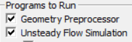

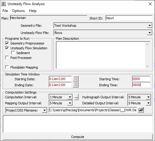
Then set your time window. Your Starting Date and Time should be the same you selected for the Fixed Start Time in the flow editor. Set your Ending Date and Time for 6 hours later.

14. Select Time Step(s)

It is appropriate to use the Courant Condition to select your time step. We are using 10 m cells. You will have to assume a velocity. You can update the velocity after you have results, but we are also going to use the automated time step tool, so this will only be a starting point.
What is a good starting time step for this project? _______ seconds
The Courant Condition is: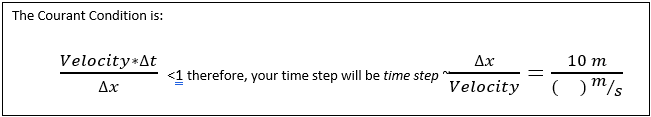

Because this whole event takes less than 6 hours, you will also want to update the output time steps: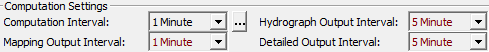

1 Hour output time steps will only provide a handful of results after your simulation. For a short model like this, these can be <1 minute without generating unwieldly results files.
But this model will have highly variable velocities. At the peak flows, the water/debris will rush down a steep canyon. But at the end of the model, it will creep along the flat alluvial plain. Therefore, it makes sense to use an automated, variable, time step.

15. Run Simulation

Back at the Simulation (Plan) editor press the Compute button.

The model may report some "max iteration" errors. Notice the Error associated with these. Do these seem acceptable for an expedited analysis?

While the model is running, you can open mapper, select the 2D Area associated with your geometry in the tree and press CTRL-F to find the cell that has the maximum error.

16. View Clearwater Results

At the end of the simulation Open RAS Mapper.
Navigate to Results on the mapper tree. You can click on the Depth, Velocity, and/or Water Surface Elevation (WSE) variables to get the max values at each cell (over the whole simulation) or you can animate the results with the time scroll bar in the upper right of mapper.
We did not design this mesh for clear water flow (e.g. we did not add a downstream boundary condition). What happens to the water when it reaches the west edge of the mesh?
Next you are going to add concentration and non-Newtonian Parameters.
How do you expect the inundation area to change? ______________
How do you expect the depth to change? ______________
How do you expect the velocity to change? ______________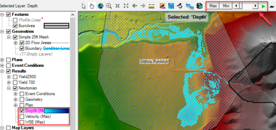

17. Add Bingham Parameters (Lowest Expected)

Next, we are going to turn on the non-Newtonian methods, add concentration, and add define non-Newtonian parameters. In an expedited analysis (or, even in a more detailed analysis) you will not have detailed estimates of these parameters.
Therefore, we will use the simplest model (Bingham) to minimize the parameters and keep them as physically based as possible. And we will bound the likely outcomes with a reasonable range of parameters (in this case t_y~700-2,500 Pa).
Open the unsteady flow file to enter flow data. Press the Unsteady flow button or select "Edit → Unsteady Flow Data..".
Save As to make a new flow file which retains the clear water flow data but adds the mud and debris approach and parameters.
Give the new flow file a name like (ty=700Pa or Yield=700) because this is the run with the lowest expected values. You will create another file with the highest.
The mud and debris capabilities in HEC-RAS are "fixed bed" sediment tools, which means you do not need a sediment file.
The non-Newtonian information is part of the flow file. To enter these data select the *OptionsNon-Newtonian Parameters…* menu from the unsteady flow editor.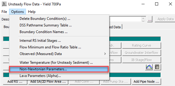

Select the Bingham Method from the Non-Newtonian Method drop-down box at the top of this editor.
That will make the appropriate parameters active.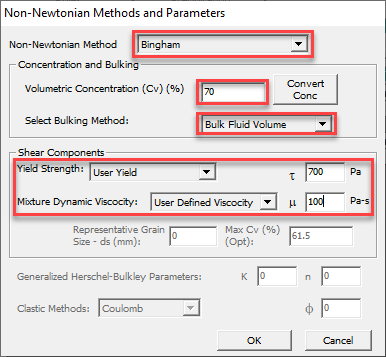

The flow data provided came from the US Forest Service spreadsheet tool. These are clear water flows, so the debris flow analysis needs to account for the volume of the sediment and debris.
During the project the USGS estimated the volumetric concentration. We will use 70% for this workshop.
Under Concentration and Bulking specify a Volumetric Concentration (Cv) of 70% and select Bulk Fluid Volume under Select Bulking Method.
Note: If you do not have an HMS model, Cv becomes another parameter you estimate and maybe run with min and max expected values.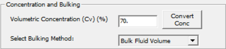

Next, define the Bingham Parameters. Switch the methods for both yield and viscosity to User Specified. As a reminder, this is how the viscosity and yield fit into the Bingham Plastic Model: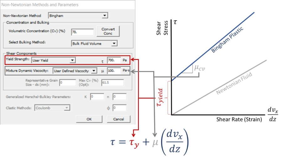

Give the model a User Yield value of 700 Pa and a User Defined Viscosity of 100 Pa-s.
Press OK to close the editor and Save the Unsteady Flow Data.
Open the Unsteady Simulation editor to create a plan. Press the Unsteady Simulation (running person) or choose the "Run → Unsteady Flow Simulation" editor.
This editor should open with no name and with the new unsteady flow file in the appropriate drop-down box and all of the plan parameters you defined (e.g. time step) still populated.
"Select File → Save As…" and save the plan with the same name as the flow file (e.g. "Yield 700").
Compute.
View the new results.
When you view the new results, you may want to change the color scheme to reflect this is a debris flow.
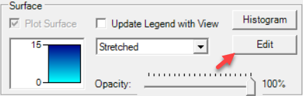
Right Click on the Depth result and select Layer Properties. Under Surface, press the Edit button.
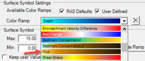
Then, from the color ramp drop-down select the Mud ramp.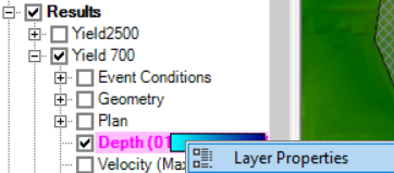

How did the results change.
How did the inundation area to change? ______________
How did the depth to change? ______________
How did the velocity to change? ______________

To view time series of both simulations at the same time, make sure the results you want to view are checked then click on the base Results node on the tree. Then Right click on the result and choose *Plot Time Series  Depth* (or whatever variable you have selected).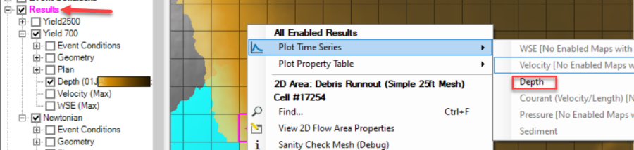

18. Add Bingham Parameters (Highest Expected)

Repeat the previous step with one change.
Create new flow and plan files with a yield strength of 2,500 Pa (instead of 700).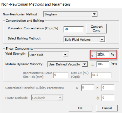

How did the results change.
How did the inundation area to change? ______________
How did the depth to change? ______________
How did the velocity to change? ______________

How sensitive are the results to the expected range of Yield Strengths?
___________________________________________________________
Try to plot a time series of all three depth results at one cell.
Turn on all depth results, and then select one so it turns pink.
Then right click on a cell and choose "Plot Time Series → Depth (see figure)"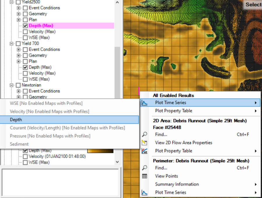

Explore the depth differences at different locations.
How does depth change with rheological parameters?
____________________________________________________________
______________________________________________________________
Smooth are the depth time series?
Do they look like they are encountering some instabilities?
______________________________________
What are some ways you could improve this model?
______________________________________

If you have extra time, experiment with the sensitivity of Cv and viscosity.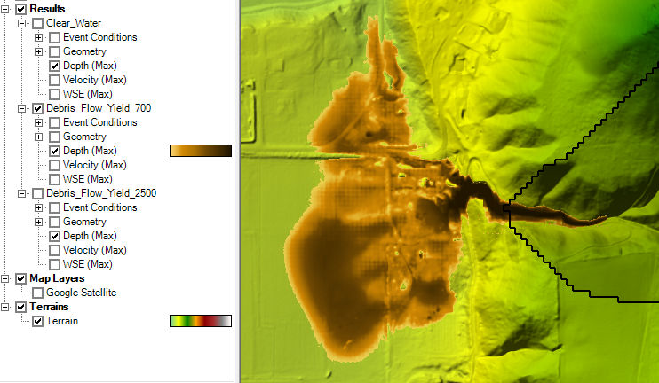

A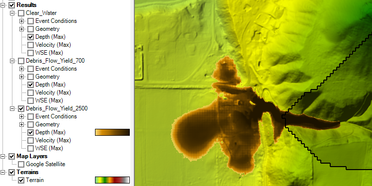

If you would like to continue to refine your model, this workshop will walk you through some steps with the data in the spread sheet: