Download PDF
Download page "Fixed Bed" 2D Sediment Modeling.
"Fixed Bed" 2D Sediment Modeling
| Starting Files | Starting Files for Part 3 Hydraulics Complete | Final Example Data Set/Solution |
|---|---|---|

Note: Video Starts with a Working Hydraulic Model
The video picks up the tutorial with a complete 2D hydraulic model, which begins in Part 3 of the tutorial below (which starts with a terrain and mesh and walks through some basic hydraulic boundary condition steps).
If you would like to follow the video and only do the sediment portion of this tutorial, start with the "Starting Files for Part 3 - Hydraulics Complete" above.
Introduction
Sediment computations add run time to hydraulic models, sometimes making sediment runtimes substantial. Two-dimensional sediment models can take even longer to run. The sediment computations for multiple grain classes are computationally expensive, and a well-designed sediment model can increase model run time by an order of magnitude or more over a hydraulic model.
HEC-RAS includes a range of modeling options that offer tradeoffs between run time and feature richness. HEC added fixed bed sediment modeling modes as intermediate analysis options. Because much of the run time in the mobile-bed sediment model is in the bed mixing and elevation updates, a fixed bed sediment capacity tool can provide some of the sediment process insight at a fraction of the runtime.
The capacity-only option is a fixed-bed, 2D, sediment model that computes sediment capacity without sediment transport while the concentration-only model solves the AD equation without bed change. Both simplifications can provide some of the value of a 2D sediment model for an intermediate level of effort (and run time) and make good screening level tools. This workshop will introduce some of the important hydraulic variables you can view without a sediment model and then introduce the fixed-bed sediment modeling options.
Warning: Models for Educational Use Only
The models in this demo are intended for pedagogical purpose only. They have been simplified and modified to fit into a brief workshop and should not be used for scientific or engineering analysis. This workshop also reflects the quickest steps to get a result, not the best modeling practices.
Objective
This reach was a depositional zone for years, requiring more dredging than any other reach in this large sand bed river. (Here is a Video of the reach).
Then the District added four structures that increased the transport capacity, and this reach has not required dredging since. We will model a rising hydrograph with and without the structures and compute the difference in capacity to develop an understanding of how these structures affected capacity.
Part 1: Add Boundary Conditions, Enter Flows, and Run Model
1. Open the workshop model.
The model has a geometry and mesh like you created in the previous workshop, a flow file, and a plan file ready to go. But it needs flow boundary conditions.
2. Add Boundary Conditions in Mapper:
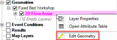
Open RASMapper Right click on the Fixed Bed Workshop Geometry and start editing.
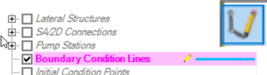
This will expand the geometry tree and make the Boundary Conditions Lines available.
Click in the Boundary Condition Lines node and select the drawing tool.
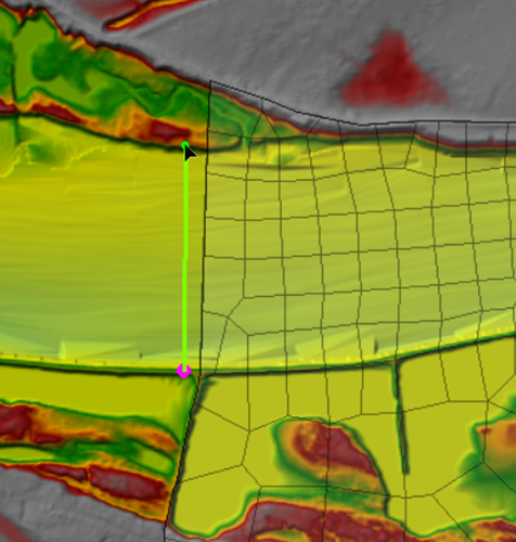
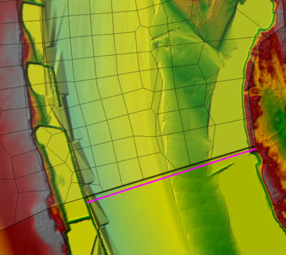
Draw boundary conditions lines Left-to-Right looking downstream (river flows from northwest to southeast) across the channel just outside the upstream and downstream mesh boundaries.
Give them intuitive names (e.g. US BC and DS BC).
Think about what portion of the channel will be actively conveying, this is the portion you want to cover with your boundary locations.
Next, you need to copy these boundary conditions to the other geometry to make sure they are identical (because they will be sharing a flow file).
Right click on the Boundary Conditions Line node on the tree and select Copy All Features.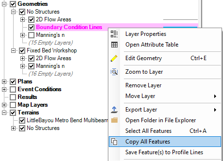
Select the other Geometry File, and press the Pencil ![]() to start editing.
to start editing.
Select the Boundary Conditions Line and select Paste Features.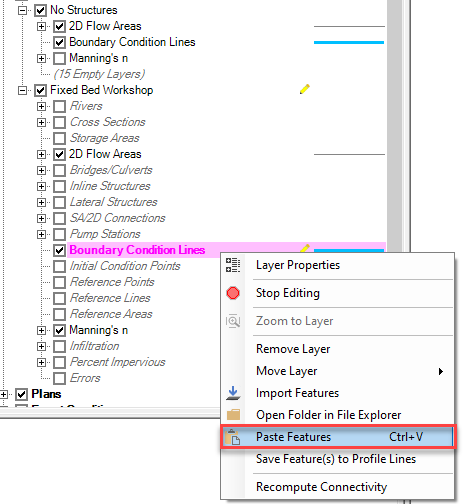
Press the stop sign to stop editing.
3. Define Flows and Stage:
We developed a downstream stage rating curve for a low Mississippi stage from the 1D steady flow model. These data are in the DS Rating Curve Tab of the Workshop Data.xlsx file.
| WSE (ft) | Flow (cfs) | WSE (ft) | Flow (cfs) | |
| 162 | 0 | 182.05 | 260000 | |
| 162.37 | 10000 | 183.34 | 310000 | |
| 164.5 | 30000 | 184.9 | 360000 | |
| 169.19 | 70000 | 186.7 | 430000 | |
| 177.03 | 150000 | 187.36 | 480000 | |
| 178.16 | 175000 | 190.47 | 625000 | |
| 178.63 | 185000 |
The files already come with an unsteady flow file (that can be shared between the geometry flies) and two plan files with some hydraulic options and parameters already set.
Open the unsteady flow file ![]() from the main HEC-RAS window and select the downstream boundary condition. Press the Rating Curve button and add the rating curve data.
from the main HEC-RAS window and select the downstream boundary condition. Press the Rating Curve button and add the rating curve data. ![]()
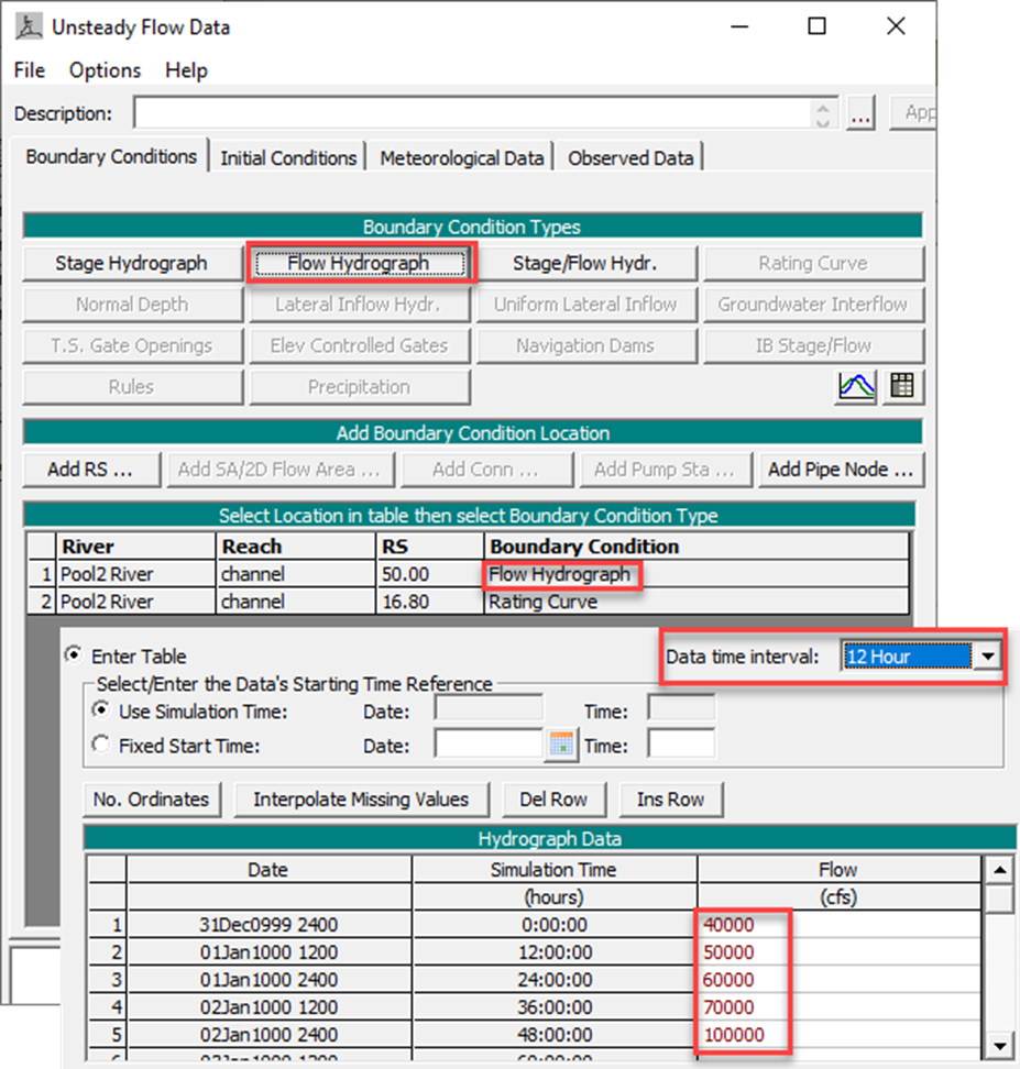
Then select the upstream boundary condition and choose the Flow Hydrograph. Choose a series of flows between 30,000 and 120,000 cfs at 12 hour increments to simulate a series of rising flows. (Note: We will work with with warmup and intial conditions in a future workshop, but they are set for you in this one).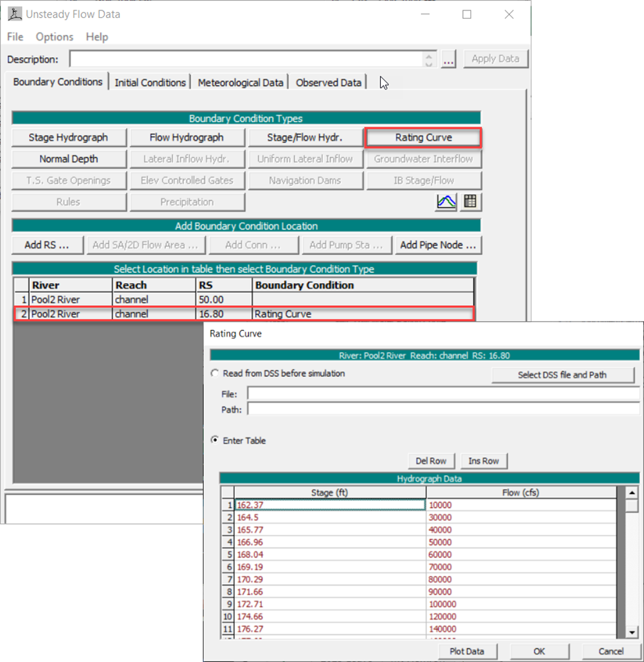
Set your energy grade slope to distribute your upstream flows to 0.0004.
Because both plans share this flow file, you only need to enter these data once.
4. Open Plan and Simulate:
Open the unsteady flow simulation editor (to the "Capacity Only (with Struc)" Plan which includes Structures) and adjust the time window to accommodate your flow series.
This plan file has warmup parameters and other features already defined.
Then press the Compute button to simulate.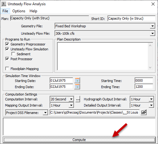
Part 2: Plot Sediment Related Hydraulic Variables (Velocity and Shear Stress)
5. Map Velocity:
Open RAS Mapper and Select the velocity results.
Plot the velocity time series at several location.
Try plotting velocity for cells and cell faces.
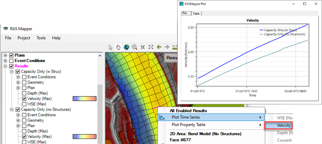
(Note: In the plot above we set the velocity color ram between 0 and 6 ft/s in the layer properties for both results, and set Opacity to ~50% by right clicking on the Velocity result and selecting Layer Properties).
6. Map Two Different Shear Stress Results:
Shear Stress is an important hydraulic variable for a range of sediment transport analyses, and can be a useful heuristic for sediment processes if you only have a hydraulic model.
But there are a couple ways to get Shear Stress results from RASMapper that are worth exploring.
Select the shear stress output in your current simulation.
Right click on the Result and select Create a New Results Map Layers. ![]()
Then expand the Hydraulics tree and select Shear Stress. Map shear stress and try to plot a time series of shear stress at a cell or a face.
Can you plot a time series of Shear Stress?____________________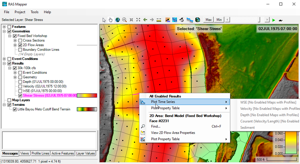
The hydraulic shear stress parameter is computed on the fly from hydraulic results, so there are no stored shear stress values. To plot a time series of shear stress, you have to request shear stress output.
7. Request Shear Stress Output:
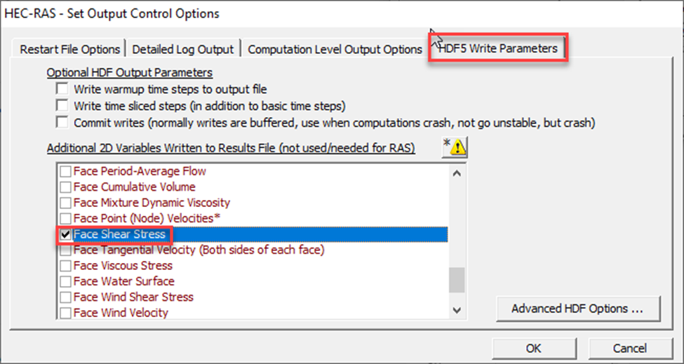
To request output that do not come standard with a RAS run, open the unsteady flow Computation Window, and select the OptionsàOutput Options menu.
Select the HDF5 Write Parameters. There are a number of very helpful features on this tab, but in particular, you can choose to write several additional 2D variables.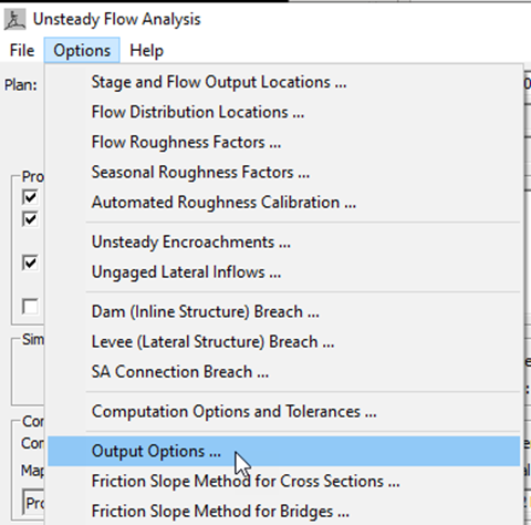
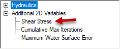
Re-run your result. After your new simulation, right click on the result in Mapper again, and choose Create a New Results Map Layers again.![]()
But this time expand the Additional 2D Variables section. You will find the new Shear Stress result under there. Select it and press Add Map. ![]()
Now you have two shear stress maps. The new Shear Stress map has default units that are not very informative. You can copy the units from the other Shear Stress Map.
Right Click on the on-the-fly shear stress result and open Layer Properties.

At the bottom of the Layer Properties editor, press the Copy Symbology button. ![]()
Next, right click on the new Shear Stress result, and select Layer Properties and Paste Symbology. ![]()
Now plot the shear stress time series by right clicking on the map. Try clicking on cells and cell faces.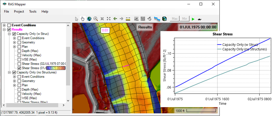
What do you notice about shear stress through this reach?
Part 3: Set Up Sediment Model
To use the capacity only, fixed bed sediment features, you still need to set up a full sediment model, which means you will need a sediment file, gradations, and a sediment boundary condition (even though you will not use the latter).
8. Open the Sediment Data Editor:
Either select the Edit→ Sediment Data menu or use the sediment data button. 
9. Select Sediment Equations:
We recommend starting with one of the 2D transport equations.
You have to scroll down to find the 2D equations in the Transport function list.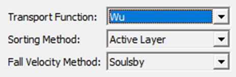 Note: It does not matter what sorting method you choose, 2D sediment will always use a customized version of the Active Layer approach, but it is good practice to select it.
10. Estimate Bed Gradation:
Fixed bed sediment models partition transport capacity by grain class like a mobile bed model, so sediment bed gradations are the minimum data requirement.
This river has 35 bed gradation samples from September 2003. These samples are plotted with river station (light blue-downstream/dark blue – upstream) in the following figure.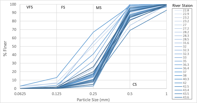
These data are also in the Bed Gradation tab of the Workshop Data.xlsx file.
Do the data have a clear longitudinal trend? ___________
How many grain classes do you think you need to represent the bed material load in this system? ___________
In this model, we used a simplified bed gradation layer, that attributes one bed gradation with the whole model.
Estimate the percentage you would associate with each grain class (and convert it into % Finer):
In this model, we used a simplified bed gradation layer, that attributes one bed gradation with the whole model. Estimate the percentage you would associate with each grain class (and convert it into % Finer):
| Grain Class | % | % Finer |
|---|---|---|
| Very Fine Sand (VFS) | ||
| Fine Sand (FS) | ||
| Coarse Sand (CS_ | ||
| Very Coarse Sand (VCS) |
11. Enter Bed Gradation:
In the Sediment Data Editor, press the Define/Edit Bed Gradation button to enter your bed gradation.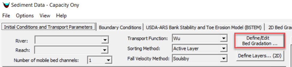
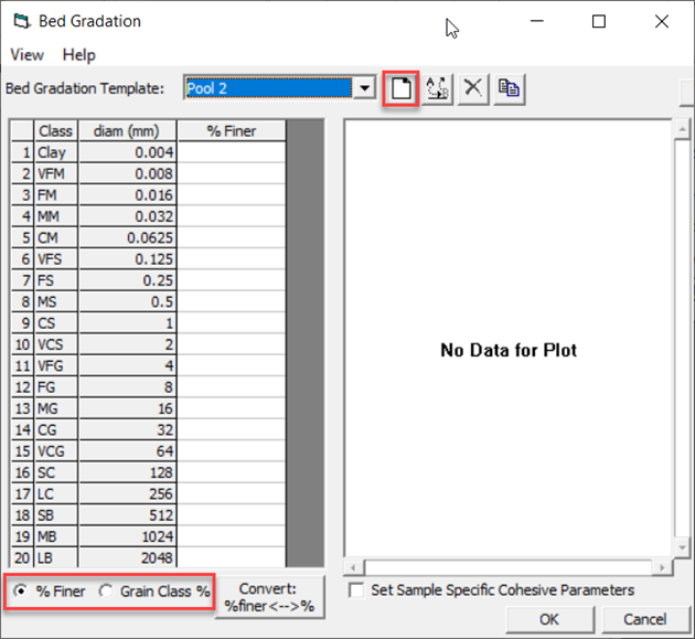
This will launch the bed gradation editor. Press the New button ![]() to create a bed gradation and give it a descriptive name. Then enter the data.
to create a bed gradation and give it a descriptive name. Then enter the data.
You can enter data as % Finer or the % in each grain class, which is often more intuitive. You could enter multiple gradations here, but for now, press OK when you are done.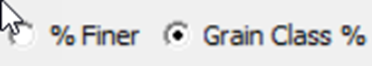
12. Associate Bed Gradation:
After you create your bed gradation, you must associate it with the Bed Gradation Layer in Mapper.
We have already created a simple Bed Gradation layer in mapper and associated it with the geometry.
So all that remains is associating the gradation you just entered with the only polygon in this layer.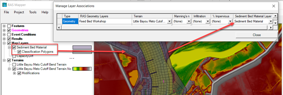
Select the 2D Gradation tab in the Sediment Data Editor.
This editor lists all of the gradation types listed in your Bed Gradation Layer (in this case there is only one, but if you had more gradations they would all appear in this list).
Click on the blank field next to the Bed Material Type.
This will give you a drop down list of all the bed gradations you have entered (again, just one in this case) and another option that is always available (Non-Erodible Surface).
Select the gradation you just created.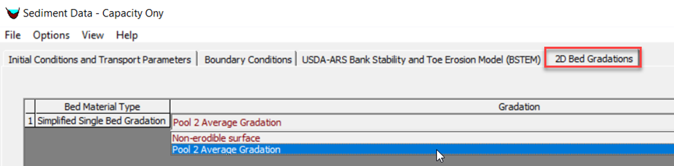
Note: If your gradation does not show up in the drop down list, try saving the sediment file and closing out. (Sometimes it even helps to close out of the HEC-RAS and reopen).
13. Select Sediment Boundary Condition:
Fixed bed sediment analysis (especially Capacity Only analysis) is not as sensitive to sediment boundary conditions.
So, for now, we will just use the Equilibrium Load sediment boundary condition.
Select the Boundary Conditions tab in the Sediment Data Editor.
The upstream boundary populates automatically.
Click on the blank field and press the Equilibrium Load button.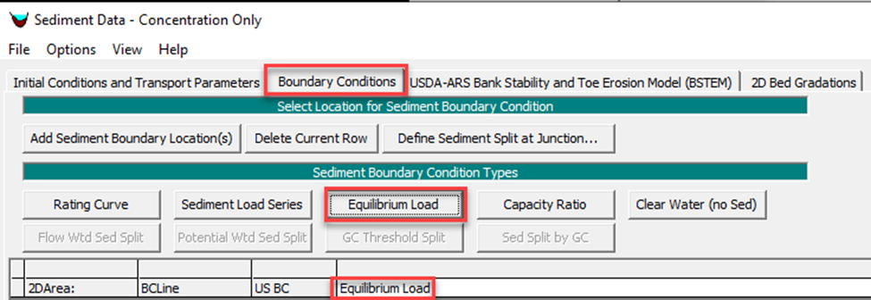
Part 4: Capacity Analysis
14. Set Sediment Model to Capacity Only Mode:
Finally, this model is currently set up for a full mobile bed analysis.
But we are not going to do that yet.
Select the Options→ 2D Sediment Options menu from the Sediment Data Editor.
Select Capacity Only from the Simulation Components dropdown box at the top of this editor.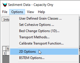
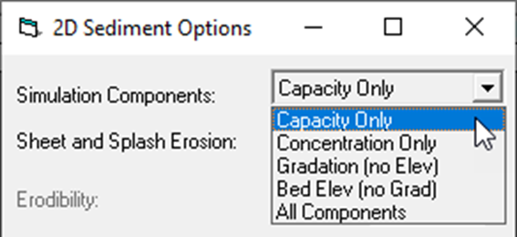 Save your sediment data as “Capacity Only”.
15. Run the Sediment-Capacity Fixed Bed Model:
Open the Unsteady Simulation editor.![]()
Save As a new plan with a descriptive name like “Capacity Only” so you will also keep the hydraulic simulation.
Then check the Sediment box under Programs to Run.
This will add a Sediment Files option to the file drop down boxes.
Select the sediment file you just created.
Then press Compute.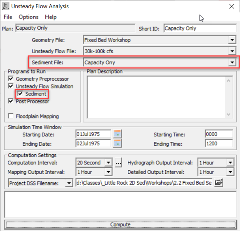
16. View the Fixed Bed Sediment Results:
Right click on the new result in RASMapper and choose Create a New Results Map Layers again.![]()
The Map Type tree has a new node. 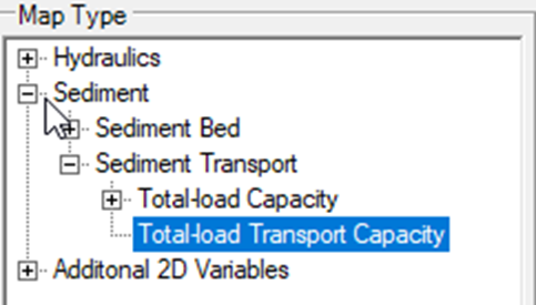
Expand the Sediment node of the results tree.
Since we did not compute bed change, you won’t be interested in the sediment bed results.
Expand the Sediment Transport node and select Total-load Transport Capacity.
Add this map.
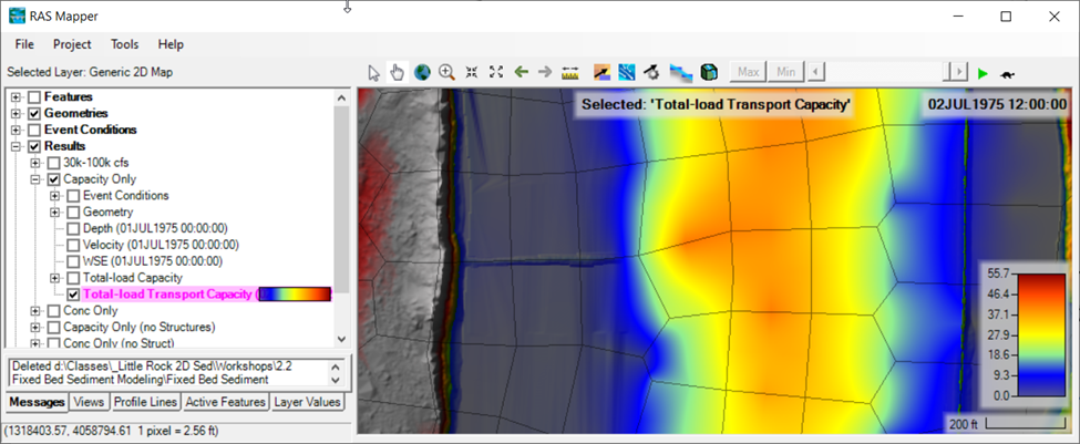
You may need to adjust the display range to the common maximum and minimum capacities.
If you adjust the alpha of the low-capacity colors, you can make them a little transparent (or adjust the Opacity bar).
Where are the highest transport capacities? _______________
Part 5: Concentration Analysis
17. Create a Concertation Analysis Plan:
Next you will experiment with the other fixed bed analysis mode.
To do that, you will need a mostly identical Sediment Data File.
Open the Sediment Data Editor and Save As.
Give it a descriptive name, like “Concentration Only”.
Then switch the Simulation Component and Save the file.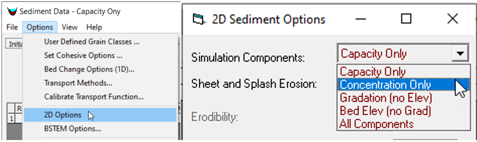
To change the Component select the Options→ 2D Sediment Options menu from the Sediment Data Editor.
Select Concentration Only from the Simulation Components dropdown box at the top of this editor.
Then Open the Unsteady Flow Simulation editor, make sure the Sediment File has changed to the file you just created.
Then save the new plan, give it a descriptive name, and press Compute.
18. View the Concentration-Only, Fixed-Bed Results:
Open Mapper and Right Click the new result to add the Concentration Result.
Expand the Sediment→ Sediment Transport node of the Map Type tree.
Total-load Concentration is now on the list.
To just add total concentration, expand the Total-load Concentration tree and select Total.
Then Add Map.
(Note: you can add results for individual or all grain classes, but this can get unwieldly at this point, so start with just the total).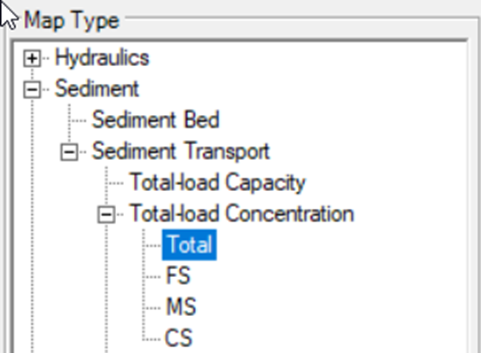
To view concentration results, you will often have to reduce the max, since local concentration spikes or initial condition effects can stretch the color band.
There are also two Concentration display options.
You might want to experiment with which works best for each map.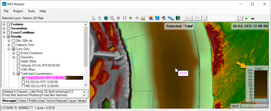
Part 6: Compare Capacity Results With and Without Structures
These results are useful to indicate relative regions of high and low capacity.
But we want to be able to weigh in on the impact of the structures.
So in this section you are going to repeat the capacity calculation on a terrain without the structures, and compare the results to try to quantify the impact of the structures before we begin mobile bed modeling.
19. Create a New Plan with No-Structure Geometry and Compute:
We have used RASMapper mods to clone the terrain and remove the four structures, reducing them to the surrounding grade.
(This video demonstrates how to remove the structures).
The project has this second terrain (which only points to the original on your computer).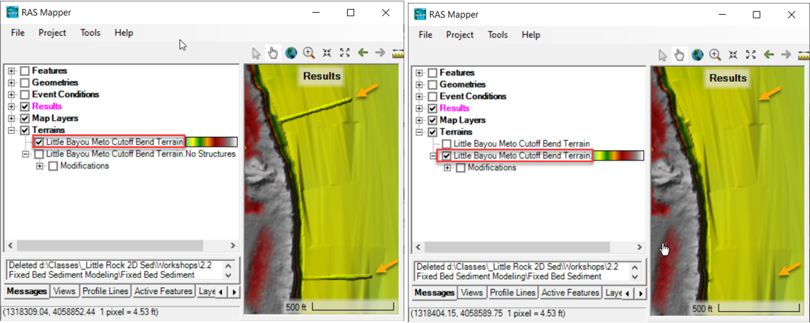
It is a little awkward to associate this terrain with a new sediment plan, however.
Terrains can only be associated with geometries.
Therefore, you will have to create a new geometry (even if it is identical) and associate the new terrain with it to run a sediment model on this terrain.
We have already done that for you.
There is a second geometry file associated with this no-structure terrain.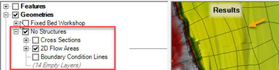
Open the Unsteady Flow Simulation Editor, save the plan as a new plan (with a name indicating it does not have the structures.
Then choose the Geometry File dropdown and select the “No Structures” geometry.
Then Save and Compute.
20. Open the RASter Calculator:
The objective of this study is to evaluate the effect of these structures.
You can view the results and set them to the same output symbology, and toggle them on and off to see differences, but that is qualitative and not particularly effective.
Instead, you are going to use to RASter Calculator to compute a map of capacity difference between the two simulations to quantify and illustrate the effect of the structures.
In RAS Mapper, select the Tools-->Create Calculated Layer option.![]()
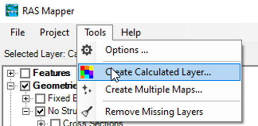
This will launch the RASter Calculator Editor (see next editor).
21. Define the Capacity Maps as Variables:
To difference the capacity results, you will have to define each capacity result Layer as a variable.
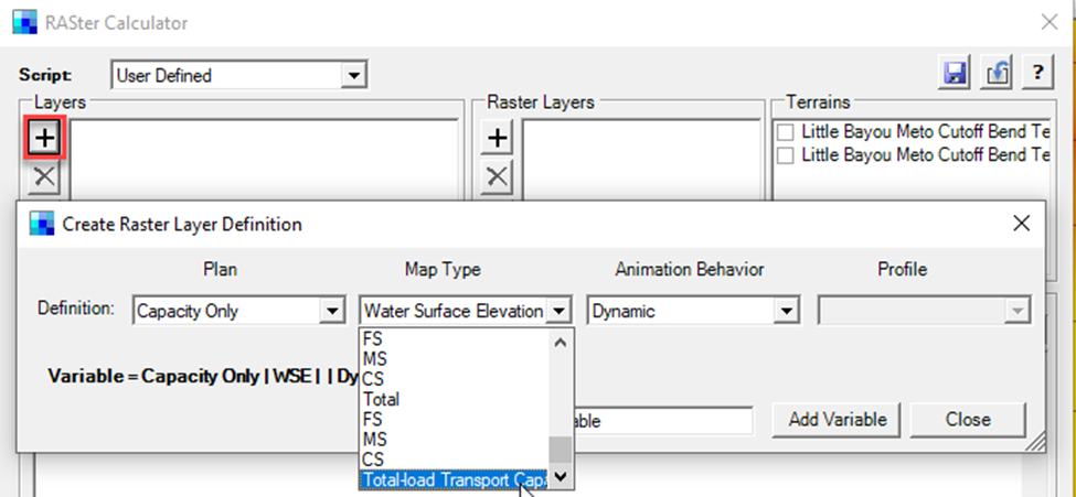
Push the Add New Layer Variable button ![]() in the top left corner of the editor.
in the top left corner of the editor.
Select the Plan and Map Type (Total-load Transport Capacity).
Leave the Animation Behavior to the default (Dynamic). 
Then give the layer a brief but descriptive variable name in the Name field (e.g. CapWithStruc). Press the Add Variable button.
This should add the variable to the Map Layer window in the upper left of the editor.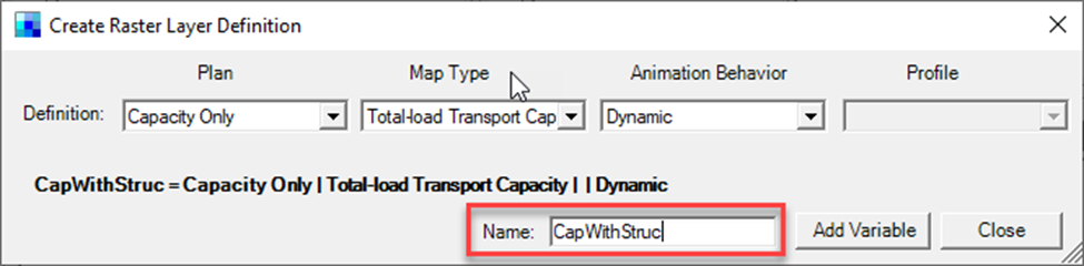
Repeat the process with the no-structure plan, and press Add Variable.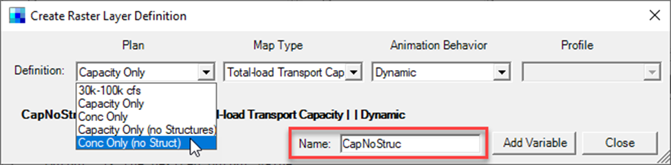
These variables should show up in the upper left corner of the editor as depicted in the following figure.
Once you add the first variable, the editor automatically populates a “stub” if-then statement to handle no-data conditions.
You are going to make the minor changes to that statement pictured below to complete the analysis.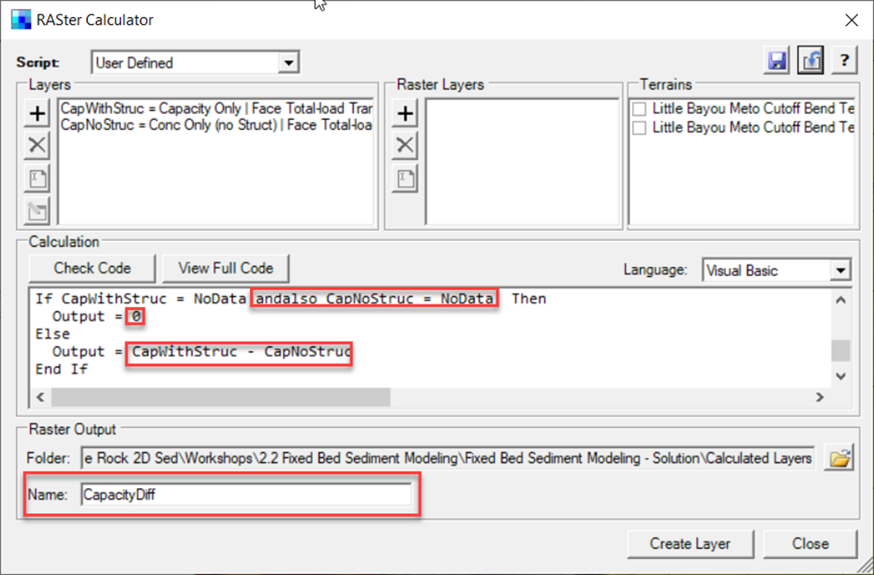
22. Write Logic to Difference Layers:
First, the data check will look at the first variable you add, but you want it to apply to both layers.
So add andalso (“Layer 2 Name“) = No Data to include it.
Then, if the NoData condition obtains, we want to set the map value to zero so we don’t compare maps where only one of them has values.
Therefore Output = 0.
Finally, in the Else statement, change the result to the difference between the layer variables.
Output = (“Layer 1 Name“) - (“Layer 2 Name“)
After you have completed the code, press the Check Code  button to see if it is complete.
If not, press the View Full Code button, which will help you find the error.
Otherwise, press Create Layer. 
23. Write Logic to Difference Layers:
The new layer will appear in the Map Layers portion of the mapper tree.
The result will import with an unhelpful 0-100 greyscale symbology.
So switch it to the Red-White-Blue “Bed Change” symbology.
I switched the red and blue to make red indicate more capacity with the structures).
If you set the Alpha of the white to zero, you will make the low-difference cells transparent.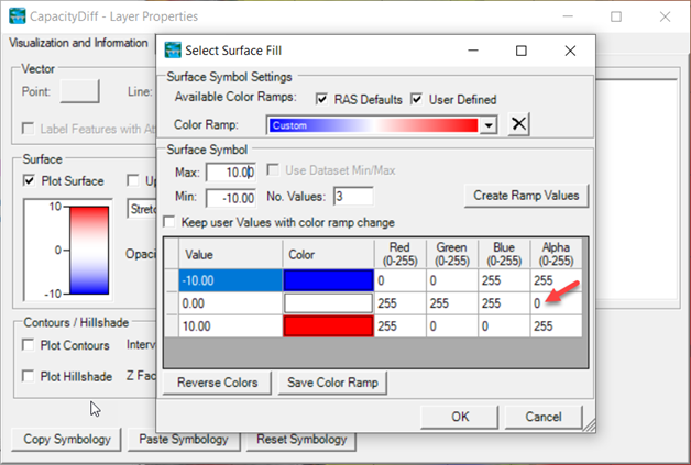
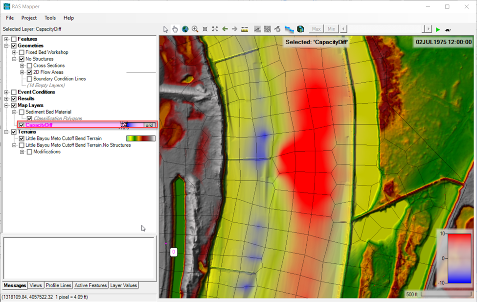
How much (%) does the capacity increase with the structures? (roughly) ________
If you have extra time: Try to make a % Change capacity map.