Download PDF
Download page Flow Hydrograph Optimization.
Flow Hydrograph Optimization
This tutorial demonstrates the approach to using the Flow Hydrograph Optimization capability for a simple HEC-RAS 2D model example application.
This is a new feature in HEC-RAS Version 6.4.

Overview
The flow hydrograph optimization capability in HEC-RAS is use to scale flow hydrograph boundary conditions to achieve a desired stage or flow at a specified location in the model. This feature can be used for both 1D and 2D unsteady flow modeling by specifying a Reference Location to be used for the optimization.
This example utilizes a simple 2D model developed for the Merced River in the Yosemite Valley. Terrain data used in this model was downloaded from the USGS NED and has been resampled. This model is not intended to be used to make floodplain management or engineering decisions, but simply to demonstrate the procedure for utilizing the flow hydrograph optimization capability in HEC-RAS. For this example, the goal will be to determine how much flow begins to flood a parking lot on the north side of the river near the Village Store.
This example will take you through the procedure outlined below.
- Identify and create a Reference Location
- Enter Flow Hydrograph Optimization information
- Perform the Flow Hydrograph Optimization simulation
- Review Results
Steps
- Open the HEC-RAS project "Example Hydrograph Flow Optimization"
Prior to utilizing the flow hydrograph optimization capability, you should confirm that the model is stable (and accurate) for a range of flows.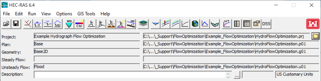
- Open the Unsteady Flow Analysis dialog.
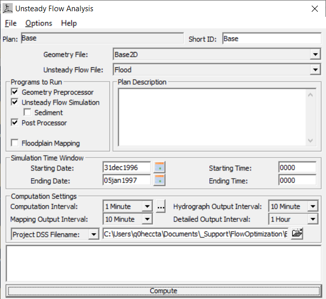
- Compute the Base plan.
- Open RAS Mapper and investigate the model to see what the computed water surface is and the Terrain elevation at the low point along the road that protects the parking lot.
Once you have identified the location of the low point and recorded the elevation, you are ready to create a reference location.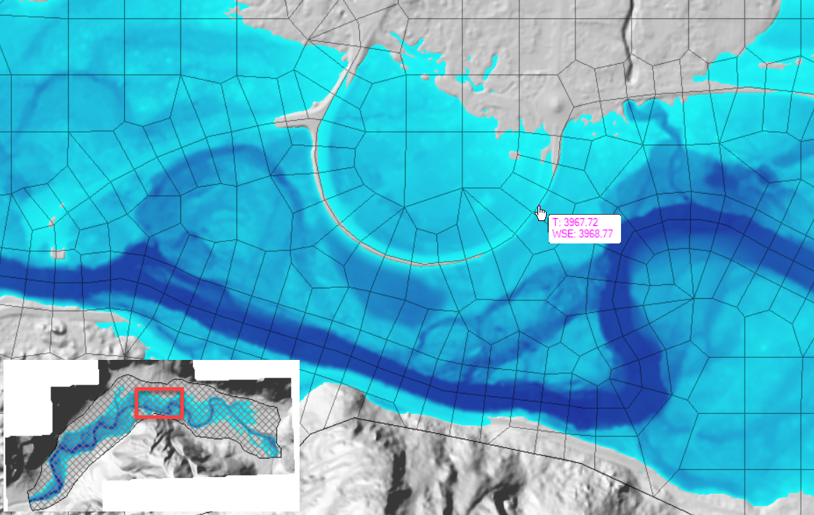
- Select the Base2D Geometry
- Start Editing
- Select the Reference Point layer
- Add a the selected reference location using the Add New Feature tool.
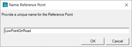
- Provide a Name for the Reference Point
- Stop Editing
Copy the Base plan using the File | Save Plan As menu item on the Unsteady Flow Analysis dialog. Provide a new name for the flow optimization plan and hit okay, in the dialog. Provide a ShortID for the new plan.
 It is not required to create a new Plan; however, by creating an additional plan, you will be able to compare results.
- Access the flow optimization data entry from the Unsteady Flow Analysis dialog Options | Automated Flow Optimization menu item.
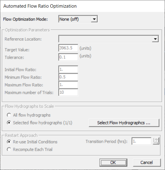
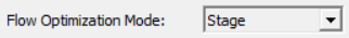
- Set the Flow Optimization Mode to Stage.
- Set the Reference Location to the Reference Point.

- Set the Target Value based the low elevation of the Terrain.
- Select the remainder of the Optimization Parameters.
The remainder of the parameters can be set as desired, depending on how you want to limit the optimization approach and number of simulations.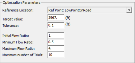
- In this example, we only have one hydrograph to scale, so you can use the All option (or select the hydrograph).
- Leave the Restart Approach to the default method.
- Press OK to save the optimization information.
- The Unsteady Flow Analysis dialog will now show a quick link that Automatic Flow Ratio Optimization has been enabled.

- Compute the Optimization plan.
As the plan runs, you will be provided a status on the Trials.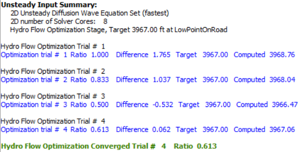
Evaluate results using the Hydrograph Plot
To compare results at the Reference Point, you will need to re-run the Base plan. (The Reference Point is new to the Base run.- From the Hydrograph Plot, choose the Type | Reference Point
- Select the Options | Plans menu item
- Select the Base plan to compare against
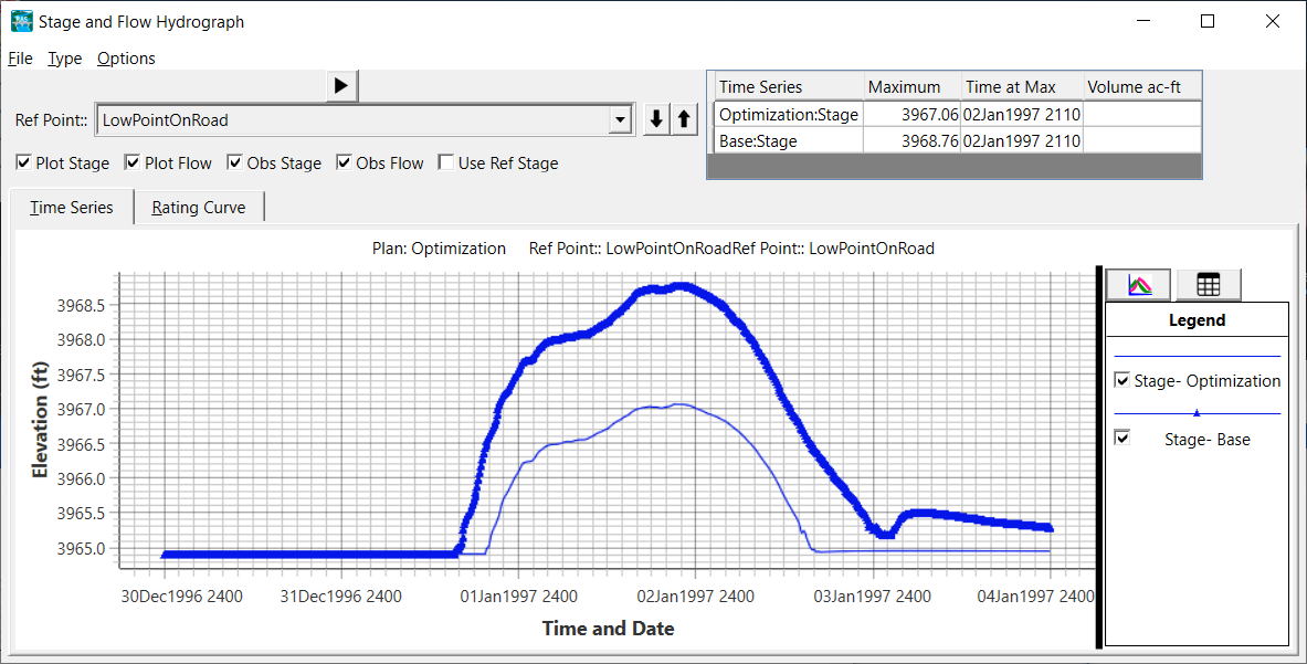
Note from the output and the hydrograph plot, the Optimization did not quite get to the desired Stage (even though it was within the specified tolerance). Therefore, if you truly did not want the water surface higher than specified Target, you may need to lower the Target by the tolerance. This will be variable on how the flow optimization final solution approaches the desired Target.
Open RAS Mapper to evaluate results
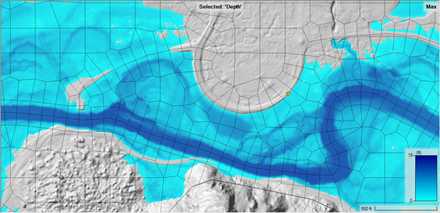
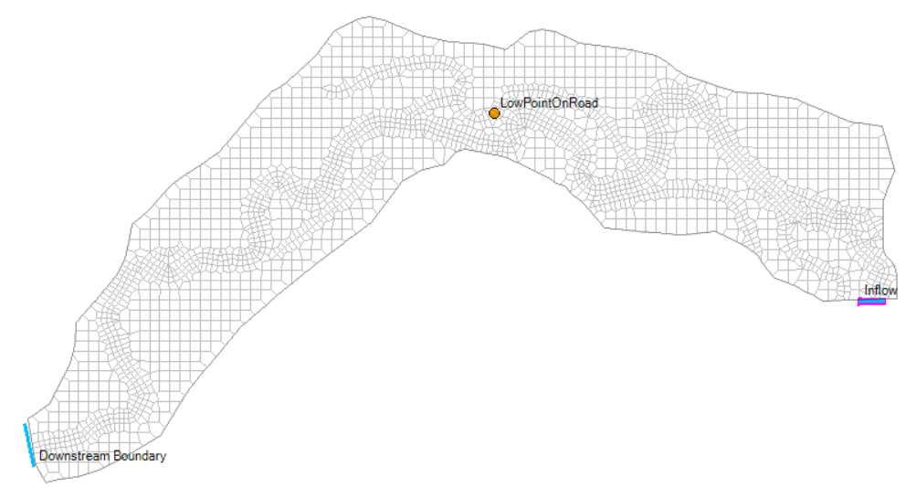
Note that the flow optimization was able to successfully scale the hydrograph to keep the desired location dry.- To access the Trial results, expand the Plan node to the Flow Optimization layer. The Flow Optimization layer can be used to identify the Reference Location and the hydrographs that were scaled. All boundary conditions are shown. Those that were used in the analysis ("Inflow" in the figure below) are shown in the highlight color (magenta).
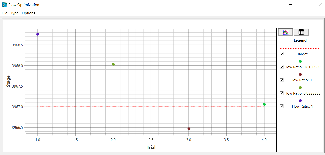
- Right-click on the Flow Optimization | View Flow Optimization Plot to show you the optimization results for the Flow Ratio and Target by Trial.