Download PDF
Download page Pipe Networks - Klawitter Pond 2D.
Pipe Networks - Klawitter Pond 2D
This tutorial demonstrates how to create a simple pipe network from existing GIS data and integrate it with a 2D surface model in HEC-RAS.
This tutorial is intended for version 6.7 Beta and forward.
Data Files
You will be working with data from an area called Klawitter Pond, located within the Valley Branch Watershed District (VBWD) in Minnesota, east of the Twin Cities metro area. Files for the tutorial are provided below:
Objective
In this tutorial, you will learn how to setup a simple pipe network and 2D surface model by importing existing GIS data. You will learn how to import and establish a 2D mesh from existing SWMM data, import conduits and nodes, and run the model/view results.
The data provided in this tutorial is from project work completed by the U.S. Army Corps of Engineers (USACE) St. Paul District for the Valley Branch Watershed District (VBWD), located in Minnesota. The data is used with permission from the VBWD for HEC-RAS Pipe Networks testing and tutorial purposes. Some of the data within the tutorial data set may have been altered specifically for purpose of testing and creating this tutorial. The data does not reflect actual existing conditions at the location. Data in this example should not be used for any other purpose than this tutorial.
Setting Up the Project
This task will setup the project, its projection, and add some of the additional reference data including the terrain and web imagery.
- Start HEC-RAS 6.7 Beta and create a new project (File | New Project). Title the project "KLW_2D" and save it in the Klawitter_2D_Tutorial folder.
- Open RAS Mapper.
- Set the projection (Project | Set Projection) using one of the shapefiles found in the Imports folder (Nodes or Conduits).
- Add an Existing RAS Terrain using KLW_Terrain.hdf located in the Imports folder under Terrain.
- Next Add Web Imagery under the Map Layers (e.g., Google Hybrid) and set the opacity of the layer to 30%.
- Next Add an Existing RAS Layer | RAS Classification Layer under the Map Layers. The LandCover.hdf layer can be found in the Imports folder, under Land Classification. This layer contains the roughness for the 2D mesh.
- Lastly, Create New Geometry under the Geometries. Name the new geometry “KLW_2D_g”. The geometry should be associated (Geometries | Manage Geometry Associations) with the terrain we just imported and the Manning's n should be associated with the LandCover that was just imported.

Creating the 2D Mesh
A single 2D Area will be imported and used as the surface model in this tutorial.
Importing the 2D Perimeter & Breaklines
- Begin an editing session in RAS Mapper for the new geometry.
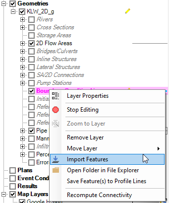
- Expand the 2D Flow Areas layer group, right-click on the Perimeters layer and select Import Features.

- Select the shapefile “Perimeter.shp” located in the included Imports folder and select Import. The polygon will be used as the 2D Area perimeter.

- Right-click on Breaklines and select Import Features. This domain was already delineated into subcatchments which we will use as breaklines to refine the 2D mesh.
- Select the shapefile "Breaklines.shp" located in the Imports folder and select Import.
Using subcatchment boundaries is a great place to start, but further mesh refinement should be considered depending on size and detail required for the project.
If you have an existing SWMM model, the SWMM *.inp file can be imported directly in RAS Mapper and converted into a RAS geometry. An advantage of importing the SWMM geometry is that HEC-RAS can automatically merge the catchments together to form the 2D Area perimeter, and automatically create breaklines along the adjacent/overlapping subcatchment boundaries. This functionality can be found by right-clicking on the geometry and selecting Import SWMM Geometry.

Generating Mesh Points
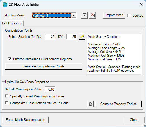
- Right-click on the 2D Flow Areas and select 2D Flow Area Editor.

- Set the point spacing to 25 as shown below and click Generate Computation Points. Close the window. You should see a computational mesh with 25 foot spacing and aligned along the catchment boundaries (breaklines).

Importing Pipe Networks from GIS
There are two important things to know about how to import conduit data into HEC-RAS:
- As is the case in all 2D stormwater modeling, conduits should reflect the true spatial extent of the pipe. Therefore, the endpoints of the conduits in the model should reflect the actual ends of the real-world conduits. This ensures accurate interaction with the 2D surface grid.
- Second, all conduits need to have nodes at their endpoints. These nodes can represent a variety of structures (e.g., manholes, drop inlets, etc.) or they can represent no structure at all (e.g., day-lighting pipes such as culverts). What the node represents is reflected in its Node Type which is inferred from the nodes attributes.
Importing Nodes from GIS
- Enter an edit session and expand the Pipe Networks layer group. Within this group is the Nodes layer.
- Right-click on Nodes and select Import Features.

- Select the shapefile “Nodes.shp” located in the included Data folder.
- Map the shapefile attributes to the HEC-RAS Pipe Network Attributes by using the table below and dropdowns at the bottom of the importer. All other attributes can be left as None.
RAS Nodes Attribute
Nodes Shapefile Attribute
Name
NAME
Invert Elevation
INVERTELEV
Base Area
BASE_AREA
Terrain Elevation Override
RIMELEV
Drop Inlet Elevation
INLET_ELEV
Drop Inlet Weir Length
WEIR_LEN
Drop Inlet Weir Coef
WEIR_COEF
Drop Inlet Orifice Area
ORF_AREA
Drop Inlet Orifice Coef
ORF_COEF

- Click Import to bring the data into RAS Mapper.
Following the import, all of the nodes should show up with a Node Type of Error (a red dot). This is because RAS cannot determine the Node Type until the conduits are imported. We will do that next.
Importing Conduits from GIS
- In the same editing session, under the Pipe Networks layer group, locate the Conduits layer.
- Right-click on Conduits and select Import Features.

- Select the shapefile “Conduits.shp” located in the Data folder. below
- Map the shapefile attributes to the HEC-RAS Pipe Network Attributes by using the table below and dropdowns at the bottom of the importer. All other attributes can be left as None. Some fields will be auto-populated, and others will get modified in the next steps.
RAS Conduits Attribute
Conduits Shapefile Attribute
Name
NAME
Mesh Cell Length
MAXCELL
Shape
XSECTION
Rise
GEOM1
Span
GEOM1
Manning’s n
ROUGHNESS
US Offset
INOFFSET
DS Offset
OUTOFFSET
US Entrance Loss Coefficient
ENTLOSSCO
DS Exit Loss Coefficient
EXITLOSSCO
US Backflow Loss Coefficient
ENTLOSSCO
DS Backflow Loss Coefficient
EXITLOSSCO

- Click Import to bring the data into RAS Mapper.
- Next open the newly imported conduit attribute table by double clicking Conduits in the RAS Mapper tree.
- Select the System Name column, then select the drop-down box, click on Selected Area Edits | Set.


- Set the System Name to “Klawitter.” Using this process, you can set attributes for the selected cells.
- Select the System Name column, then select the drop-down box, click on Selected Area Edits | Set.
- Stop the edit session and Save the geometry edits.
Upon close of the edit session, RAS Mapper will perform data checks on the pipe network and create a pipe mesh if there are no problems. If you zoom in on the network, you will see individual cells, based on the conduit Mesh Cell Length attribute. You will also see cells at nodes that represent manholes.
Boundary Conditions
HEC-RAS has several boundary condition types for introducing and removing flows from the model. In this tutorial, flows are introduced via Internal Flow Boundary Conditions inside of the 2D areas. These boundary condition lines are placed near the low point of each catchment. This is similar to a traditional stormwater (SWMM) model, in which runoff hydrographs are fed into nodes, after which they are able to enter the pipe network. Note that an alternative approach uses a precipitation boundary condition on the 2D mesh, allowing flow to be routed on the surface and then enter the pipe network via drop inlets or culvert openings.
This task will take you through the process of adding the boundary condition lines and connecting the runoff hydrographs to the boundary conditions. For this tutorial, we will be utilizing a hypothetical 100-year, 24-hour storm event.
Adding Boundary Condition Lines
This tutorial is based on a 1D model that was originally created in SWMM. These boundary condition lines were created by using GIS to create a circular polyline around the model storage nodes (using the buffer geoprocessing tool). The result is a circular line located at the approximate low point of each catchment. When the hydrograph is linked to the boundary line, the inflow is distributed across the line and enters the model in the cell(s) that overlaps the boundary line.
The inflow hydrographs are a result of previously completed hydrologic modeling in SWMM, and accounted for hydrologic losses (infiltration, evaporation, etc.).
- Enter an edit session in RAS Mapper.
- Expand the KLW_2D_g geometry, right-click on Boundary Condition Lines, and select Import Features.
- Select the shapefile titled “2D_Inflow_BC.shp” located in the included Imports folder.
- Ensure that the name attribute is mapped to Name, and click Import. The name attribute will assign the hydrograph to the correct boundary condition line. You should see 5 circular boundary condition lines, one within each catchment, as shown below.

- Stop the edit session and Save the edits to the geometry.
Klawitter Pond - Initial Conditions
Klawitter Pond (the large depressional area to the north) is filled with water year round. You will use initial condition points to set the initial water surface elevations for the pond.
- Enter an edit session in RAS Mapper.
- Expand the KLW_2D_g geometry, highlight Initial Condition Points in the tree. Select the Add New Feature button within the edit toolbar.

- Place an initial condition point near the low point in the pond terrain, as shown below. Name it "Klawitter Pond".

- Stop the edit session and Save the edits to the geometry.
Unsteady Flow File and Initial Condition Setup
- Open the Unsteady Flow Data Editor from the main RAS toolbar.
- Save the unsteady flow file with the Name “KLW_2D_100yr_u”.
- Under the Boundary Condition window, you should see all 5 of the boundary condition lines that we added in the previous step. Additionally, if you switch to the Initial Conditions tab, you should see the initial conditions point (Klawitter Pond), listed. Set the initial condition elevation of Klawitter Pond to 955 ft. Then return to the Boundary Conditions tab.
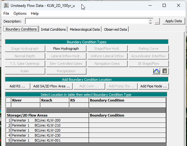

- Select the empty boundary condition for first boundary condition line (KLW-200) and select Flow Hydrograph above.

- For this tutorial, a DSS file has been setup with the inflow hydrographs. The DSS file is located in the Data folder. Begin by selecting the Read from DSS before simulation option and clicking on Select DSS file and path.

- Add the DSS file. All of the inflow hydrographs should populate. We will only be using the 100yr hydrographs for this tutorial, so sort by part F for the 100yr events. The 5 hydrograph data sets for each of the boundary condition lines should remain.

- Select the correct data set for the boundary condition line using part B and click OK on the two subsequent windows. To check to make sure the DSS file is linked properly, you can plot the data.


- Repeat the previous step for the other 4 boundary condition lines, keeping in mind the boundary condition line name and the corresponding hydrograph data.
- Save the unsteady flow file.
Plan Setup
- Open the Unsteady Flow Analysis window from the main RAS toolbar.
- Verify the Flow file and the Geometry file are properly selected.
- Name the plan “KLW_2D_100yr_p” and Save.
- Set up the plan settings as shown below:

- Save the plan and project file.
Running the Model Simulation
This task will take you through the process of running the simulation that you just set up.
- Begin by opening up the Unsteady Flow Analysis editor. Click Compute. Grab a cup of coffee. When completed the computation should look like the figure below.

There are warnings about Node Type. This is because we mapped drop inlet information to the nodes at the ends of culverts. Culverts do not require this information; it could have remained unmapped or the data could have been removed from the import shapefile.
Viewing Model Results
This task will take you through the process of viewing the various pipe modeling results.
Stage and Flow Hydrographs
In this section you will view stage and flow hydrograph data for the model run above.
Pipe Nodes
- Press the Stage and Flow Hydrograph button to view time series for stage and flow at nodes and conduits.

- Select the Type menu and select Pipe Nodes. This will open the standard Stage and Flow Hydrograph data window. Notice that there are new options at the top, associated with the pipe network. You can use the dropdown menu to select specific nodes.

- Select node KLW_J-001.
- Expand the window to include the table data as well as the graph (using the Table icon above the legend on the right side of the graph). Because node KLW_J-001 is a junction node (manhole) within the middle of the pipe run, the results provided include the stage (elevation) at the node cell, the inlet inflow into the manhole (none), the inflow into and out of the upstream and downstream pipes. Look at other nodes (of different types) in the model and you will see that node types that are culvert openings at the downstream end of a conduit (e.g., KLW-220) include stage and conduit flow out. Culvert openings at the upstream end of a conduit (e.g., KLW-200) include stage and surface flow in. All other functionality within the Stage and Flow Hydrograph window are available, including copying data from the table and adding observed data for comparison/calibration.

Pipe Conduits
- Select the Type menu and choose Pipe Conduits. This allows you to access similar results for conduits.
- Select conduit C2. Conduit data includes stage and flow at both the upstream and downstream faces of the conduit (i.e., the face where water transfers from the upstream/downstream node into or out of the node cell). Notice the initial rise in the downstream stage to an elevation of ~958.4 ft. After the hydrograph falls off, the downstream stage returns to this elevation rather than the initial downstream stage. This is because the next downstream pipe in the model is inversely (negatively) sloped, causing water to get trapped in the pipe system. You can verify this is occurring by viewing the profile results in the next section of the tutorial.

Data can also be extracted from cell faces that are internal to the pipe mesh (i.e., not the US or DS face). This can be done by right-clicking on a specific pipe mesh cell face in RAS Mapper.
Profile Plots
In this section you will view and animate profile plots for pipes in the model run above.
Viewing Conduit Profiles
- Open RAS Mapper.
- Turn on the results of the model run and make sure that all of the components of the geometry are turned on, as shown below.

- Select the Conduits layer (shown above) and, using the selection tool, select the northernmost run of pipes that drain into the pond.
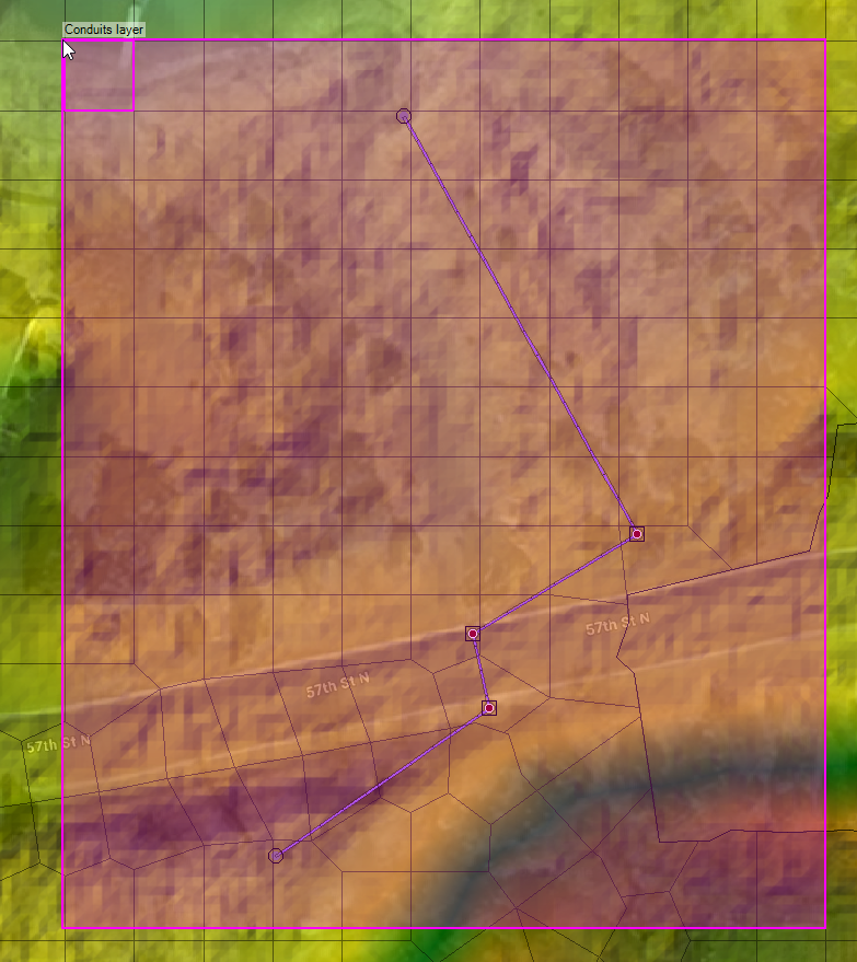
- Right-click the southern-most pipe of that group (C1) and under the menu, select Results - Profile Plot.
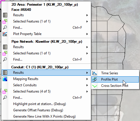
The profile plot shown below will open.
- The left side of the window lists all of the conduits in the model. The highlighted conduits are included in the profile plot. The order of conduits is plotted from downstream to upstream.
- The middle window shows the pipe profile plot on the top. As denoted in the legend, this profile plot includes hydraulic data including the energy grade line (EG), hydraulic grade line (HGL), water surface (WS), and critical and maximum water surface. It also includes the conduit outline, the grid faces within the conduits, the inlet structures, and the terrain profile.
- Below the profile plot are velocity and flow profile plots for the conduit network. As with the previous hydrograph window, tabular data can be accessed by clicking the Table icon above the legend on the right side of the graph.
- Animate the conduit profiles using the animation bar at top of the plot. The profile plot as well as the velocity and flow plots will update.
- Scroll the animation to the end of the simulation. Notice how the downstream conduit is steep enough that you have supercritical flow but then a hydraulic jumps occurs in the conduit and begins moving upstream as the tailwater rises. You will also notice water is trapped in the inversely sloped pipe section at the end of the simulation.

Viewing Saved Lists
- The Saved List tool in Profile Plot will allow you to store reference plots.
- Start by selecting the conduits you want to reference in the left window.
- Then click Edit Saved Lists, click the
 button, give your list a Name and click OK.
 - You now have a stored plot that you can go back to in the dropdown menu incase you toggle away from that plot.

RAS Mapper Spatial Results
In this section you will view the various pipe network spatial model results in RAS Mapper.
- Open RAS Mapper.
- Expand the Results of the model run.
- Turn on the results Geometry, as shown in the figure below.
- Near the bottom of the results tree, you will see four new results, specifically related to pipe model: Pipe Water Surface Elevation (WSE), Pipe Depth, Pipe Percent Full, and Pipe Velocity.

- Zoom into the northernmost run of pipes (conduits C1, C2, C49, and C50); we will look at results for these pipes.
- Begin by turning on all of the result layers in the tree (Depth, Velocity, WSE, Pipe WSE, Pipe Depth, Pipe Percent Full, and Pipe Velocity).
- Select the results layer (KLW_1D_100yr_p) as shown in the figure above. Highlighting the top of the results tree before you move the animation bar ensures that all of the results currently turned on will shift to the same timestep.
- Drag the animation bar to 01JUN1998 12:45:00 (the simulation time is shown in the upper righthand corner of the map).
You can use the Layer Values to add multiple outputs for comparison.
- Navigate to the Layer Values tab in the bottom left corner of RAS Mapper.
- Highlight the result(s) you want to add and click the
 button in the Layer Values tab.
 - Make sure the Use box is checked.
- You can also change the ID of the result for better identification.
- Using your cursor, hover over the map to view multiple results at the same time for comparison. As long as the Use box is checked the corresponding result(s) should appear even if it is not highlighted in the Results tree.
- The below image compares the Depth, Pipe WSE, and WSE values.

Water Surface Elevation (WSE)
- Turn off all the results except for the WSE and Pipe WSE. Your results should look like the figure below. Notice that the depression to the south (red) and the pond to the north (green) show constant surface elevations while the pipe run shows a gradient. This is indicative of the water surface profile running through the pipes. If you highlight either of the WSE results in the tree, you can hold your cursor over the map to see the WSE values at any point, for that result.

The Pipe WSE layer is reporting the elevation of the hydraulic grade line in the pipes.
Pipe Depth
- Turn off the WSE and Pipe WSE results.
- Turn on the Depth and Pipe Depth results.
- The results should look this the figure below, showing depth of water on the surface and depth of water in the pipe network.

Pipe Percent Full
- Turn off the Pipe Depth results and turn on the Pipe Percent Full results.
- Your results should look like those shown below. Note that the red portion of the pipe shows where the HGL is crossing the top profile of the pipe (i.e., surcharged). Feel free to highlight the top of the results tree (KLW_1D_100yr_p) and move the animation bar to see how the surcharging of the pipe system changes throughout the model simulation. At the end of the simulation, you'll see the only surcharging is at the outlet of the system. This is due to the pond tailwater backing up into the pipe system.

Pipe Velocity
- Turn on only the Pipe Velocity layer.
- Use the animation bar (with Pipe Velocity highlighted in the results tree), to see how the velocity of the water in the pipes changes throughout the model simulation. Peak velocities occur near 01JUN1998 12:30:00.

This concludes the 2D Pipe Network tutorial.