Objective

In this tutorial, you will learn how to use the geometry import tools in HEC-RAS Mapper to create a pipe network from an existing EPA SWMM model. 

This tutorial is intended for version 6.7 Beta 3 and forward.

Dataset

Download :BeaverLake-SWMM-Import - Start.zip

The data used in this tutorial is for training purposes only and should not be used for purposes other than training. Some of the data within the tutorial dataset may have been altered specifically for purpose of testing and creating this tutorial and do not reflect actual conditions at the location. 

Overview

Pipe Networks were added in version 6.6 allowing users to define stormwater networks and integrate them with existing 1D and 2D surface models. Most of the industry standard tools for stormwater modeling utilize the SWMM engine from the EPA. To make conversion of existing SWMM models to HEC-RAS easier, a SWMM import tool is included in HeEC-RAS. This import tool will take geometry information from SWMM .inp file and create HEC-RAS Pipe Networks automatically.

This tutorial starts with an existing 2D rain-on-mesh model for a small suburban watershed near Nashville, TN. An existing EPA SWMM will be imported to create the pipe network in HEC-RAS, and a simulation will be setup to run the pipe network integrated with the 2D surface. 

In order to import EPA-SWMM geometries directly into HEC-RAS, the EPA-SWMM elements must be georeferenced in the same coordinate system as the receiving HEC-RAS model.

Import SWMM Geometry

1. Open the HEC-RAS project "BeaverLakeSWMMImport"
   
2. Open the Unsteady Flow Analysis Dialog and Compute  the 25YR_2D_Only plan.
   
   
3. Open HEC-RAS Mapper  and turn on the geometry layer to see the extent and characteristics of the model domain.
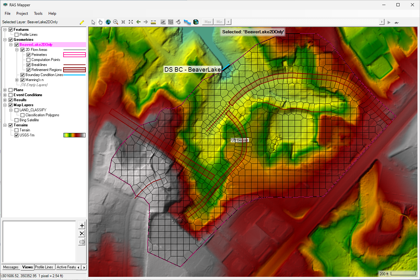   The model domain is a small neighborhood on terrain that slopes toward the downstream boundary, Beaver Lake. 2D Mesh refinements have been made to align the cell faces with controlling terrain features such as streets and berms.  Precipitation is the only inflow boundary condition, and downstream boundary at Beaver Lake is represented with a Normal Depth estimate allowing flow to leave the 2D domain.
4. Find the 25YR_2D_Only Results layer and Turn On the Depth Layer. Animate the Depth Layer to see how the watershed drains and view the Max Depth
   
5. Turing on the Velocity map layer and the Particle Tracing to get a feel for flow direction in the model.
   

Geometry Setup

1. In HEC-RARS Mapper Right-Click the "BeaverLake2DOnly" geometry and select Save As..
   
2. Name the New Geometry "BeaverLake with Drainage"
3. Start an Edit Session on the new Geometry. 
   
4. Select Import SWMM Geometry 
   
5. In the Dialog that opens click , navigate to the SWMM directory, and select the BeaverLake.inp file.
6. Next deselect the first two option in the dialog and click OK. These options allow the user to bring in the SWMM Sub catchments as HEC-RAS 2D Areas, but this geometry already has a 2D Area.
   
7. Once the import is complete, stop the Edit Session and Save. 
8. Expand the Pipe Networks (Beta) Node in the tree and turn on both the Nodes and Conduits layers.
   
   The X-Y coordinates of the SWMM Links and Nodes from the SWMM .inp file are used to create the model elements in HEC-RAS. That means that the EPA SWMM model must be in the same Coordinate Reference System as the HEC-RAS model and the model elements in SWMM must be geospatially accurate. 
   The Nodes are colored based on their Node Type. The Legend for the Node colors is displayed in bottom right corner when the Node Layer is selected in the Tree.
   
9.  Open up the Nodes and Conduits Attribute Tables.
   
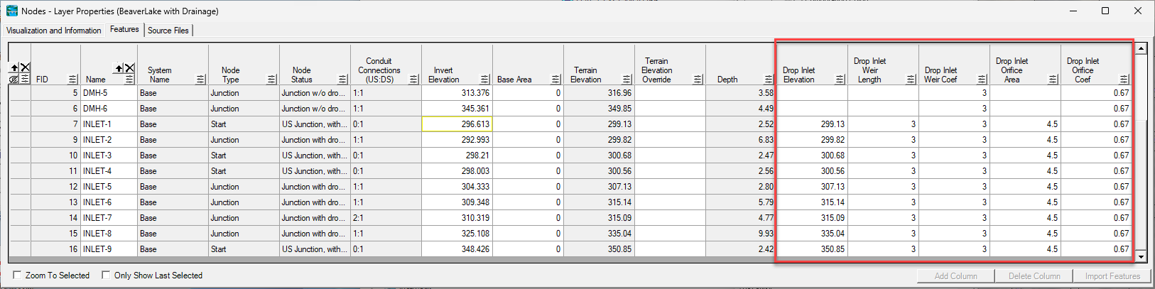
   In the Nodes Attribute Table you will notice that the Node Name and Invert Elevation Attributes were brought in from SWMM for each node.
   The gray columns are attributes that are computed by RAS and the white columns are user editable. To learn more about the Node and Conduit Attributes, see the User's Manual
   
10. Open the Conduit Attribute Table.
    Many more attributes about the conduits are brought in directly from the SWMM model including:  Name, US Node, DS Node, Shape, Rise, Span, Manning's n, US Offset, DS Offset.
    
    Note that several other attributes are computed for you including the Length of the conduit (from the the polyline), the Slope of the conduit, and US and DS Elevations (Node inverts + Offsets).
    
    Upon import, a Mesh Cell Length is computed for you based on the size of the conduit, however, usually requires later adjustment based on expected velocities and timestep.
    

SWMM Conduit Length

In EPA SWMM based models, the length of the conduit used in the computations is typically a user set attribute. That means that the line representing the conduit in SWMM is not required to be spatially accurate in location or length. This is a major difference when compared to HEC-RAS, which takes a geospatial approach to defining geometry. HEC-RAS relies on the geospatial location of the conduits and nodes for hydraulic connectivity, the length of the polyline for the computations, and the path of the polyline for the computations in the case of bend losses.

Modelers should be aware of this difference when importing model geometry form SWMM that may or may not be spatially accurate.

Modify Node and Conduit Attributes

Much of the required attributes for Conduits and Nodes have already been set from the SWMM model attributes. However, some adjustments and additional information are require to better define the Pipe Network and it's connections to the surface. 

In this section we will:

• Add Drop Inlets to Nodes
• Fix Pipe Network geometry errors
• Set Node Base Areas
• Set steep Conduits to Instantaneous computations
• Adjust Mesh Cell Lengths for Conduits

Add Drop Inlets

Drop Inlets are defined on Nodes and allow for flow to enter the Pipe Network from the 2D surface model, or  allow for flow to surcharge from the Pipe Network on to the 2D surface. Drop Inlets regulate flows into the network by using both weir and orifice equations as well as headwater and tailwater to create a family of rating curves. More on Drop Inlet computations can be found in the Hydraulic Reference Manual for Pipes.

Drop Inlet Parameters

At this time, HEC-RAS does not distinguish between different type of inlets (i.e. Curb, Grate, Combination, Depressed) in the computations, and instead is just using the basic weir and orifice flow equations to regulate flows into the drop inlets. As such, a modeler should consider the type of inlet being represented and adjust the weir and orifice parameters to account for that. 

1. In HEC-RAS Mapper start an Edit Session. 
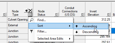
2. Open the Node Attribute Table of the Pipe Network and Sort the table by Node Name:
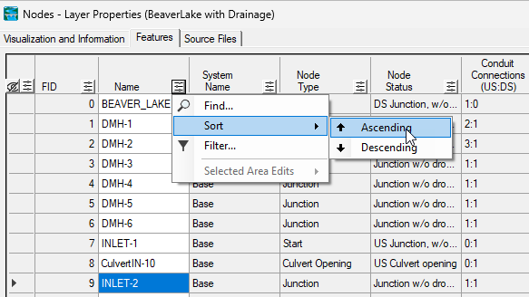   All the Nodes with "INLET" in the Name are where curb inlets are located, so we need to add a Drop Inlet to represent them those nodes in the geometry.
3. Select all the Terrain Elevation cells for the INLET Nodes and press Ctrl+C to copy.
4. Select the same cells in the Drop Inlet Elevations column and press Ctrl+V to paste.
   
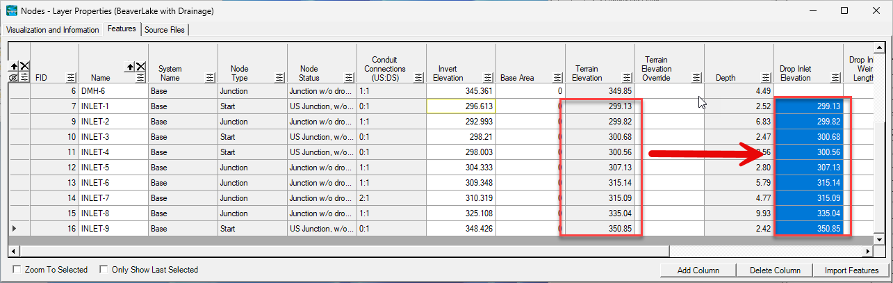
   The Drop Inlet Elevation is the elevation at which, when exceeded, water is allowed to enter the Pipe Network from the 2D cell the Node is located in. In HEC-RAS, flows into drop inlets are governed by weir flow for lower heads, and transition to orifice flow for higher heads. As such, we will need to enter parameters for both the weir and orifice equations to describe the drop inlets. 
5. Next, set the Drop Inlet Weir Length to 3 feet for the INLET nodes. A quick way to do this is highlight desired cells to change and use the Set capability as shown below:
   
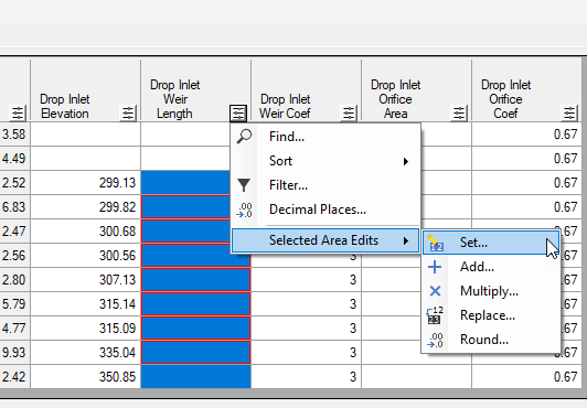
6. Following the same steps as above, set the Orifice Area to 4.5 ft² . Leave the default settings for the orifice and weir coefficients. The Node attributes table should now look like the figure below:
   
   
7. Stop the Edit Session and Save.
8. Going back to the map window, you will now see a squares around the nodes that have Drop Inlets. 
   

Fix Errors

In HEC-RAS Mapper, the Errors Layer is created upon Saving the geometry, and it is very handy for chasing down geometry issues in HEC-RAS Mapper. The Error Layer will show both warnings and errors that result when the geometry is validated upon save. 

1. In HEC-RAS Mapper, turn on the Errors Layer. You should see a few Conduits highlighted in red in the map window. 
   
   

   Note

   If no errors are detected upon geometry validation, the Error Layer will not be visible in the tree.

2. Right-click the Errors Layer and open the attribute table
   
3. The table show the same issue at three different conduits.
   
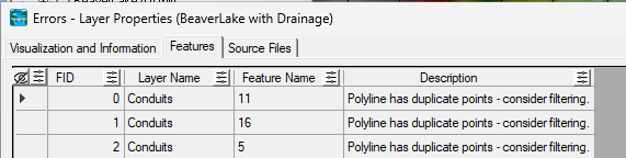
   This error resulted from how the the conduits were drawn in the SWMM model. In the model there were vertices at either end that were directly on top of the nodes which serve as the end points for the line - this made for duplicate points on ends of the line. 
   
   

   SWMM Conduit Polylines

   If conduits have been reversed at some point in the SWMM model development it can cause incorrect ordering of the vertices of the conduit polyline. When imported into HEC-RAS, this incorrect ordering can result in a conduit polyline that doubles back on itself between nodes, making for a conduit that is much longer than expected. Using the Error Layer, and the  Profile Plot to inspect the imported geometry in HEC-RAS Mapper can help identify these issues.

4. Start and Edit Session in HEC-RAS Mapper.
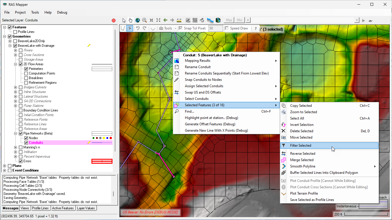
5. With the Conduit layer highlighted in the tree, select the 3 conduits in the map window by using Ctrl+Click.
6. Right-Click one of them and choose Filter Selected as shown below, and set the Filter Tolerance to 0.5 ft
   
7. Close the Edit Session and Save.
   There will be 1 additional warning in the Errors layer about the invert elevation of Culvert Opening node. This is warning the user that the Culvert Opening invert is below the invert of the 2D cell. HEC-RAS handles this case computationally, but the warning is there to ensure user is aware of this occurrence in the geometry. We don't need to address the warning for this dataset. 
   
8. Turn off the Errors Layer.

Set Node Base Area

The Base Area is an attribute on the Nodes that allows the user to represent the size of the manhole or other junction structure between conduits. When the Base Area is changed from the default value of 0, additional volume is added to the volume-elevation property table for the node to account for manholes, junction boxes, or other forms of underground storage. 

1. Open an Edit Session in HEC-RAS Mapper and Open the Node attribute Table. 
2. Sort the Attribute Table by Node Type. 
   
3. Select all the Base Area cells for Node Types of Junction and Start, then set the Base Area to a standard manhole size 12.56 ft².
   
4. Stop Editing and Save. 
   
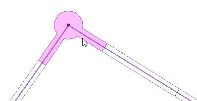
5. In the map window, zoom to a node location. You will now see the Node computation cell has increased beyond the width of the pipe to represent the Base Area
   

Plot Profile and Inspect Geometry

As you are building Pipe Network Geometry it is helpful to use the Profile Plot often to inspect the geometry for any setup mistakes. Profile Plots can be accessed from the Geometry layer in HEC-RAS Mapper, or the Results layer if you want to visualize results with the geometry. 

Note

To view the Pipe Network Profile plot for the geometry, the user must not be in a Edit Session, and must have a complete geometry with a Pipe Network Mesh.

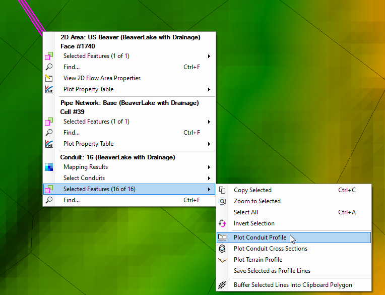
1. Outside of an Edit Session, select the Conduits layer in the tree and press Ctrl+A to select all the conduits (they should be highlighted in magenta)
2. Next Right-Click a Conduit → Selected Features → Plot Conduit Profile
   
   
3. With the map visible, move your cursor around the profile plot and watch the map window. You will see a tracer in the map window highlighting where each conduit is spatially:
   

The Profile Plot can be very useful in understanding how the Pipe Network is connected, where each conduit lives in space, where manholes and Drop Inlets are located, what the cell sizes are, and where any setup mistakes were made.

Looking at the profile plot for this geometry the modeler can quickly see that the upper end of this system is very steep (~20% slope), pushing the limits of the assumptions of the shallow water equations. Next we will mitigate that problem as well as set better initial cell sizes for the rest of the pipe Network. 

Set Conduits to Instantaneous

In some cases the modeler may not be interested in what is happening hydraulicly inside of a conduit, and instead just wants to translate inflows from Drop Inlets to the main trunk lines. This is possible by setting the Conduit Computation Method to Instantaneous and is most often used on short lateral lines. However, in this case of this tutorial dataset, we are going to set the very steep conduit to the Instantaneous method to avoid the computational burden involved with very steep pipes. To learn more about the Conduit Computation Method, see the Conduit Attribute Section of the Pipe Network Geometry User's Manual

1.  In an RAS Mapper Edit Session, Select the most upstream conduits in the Pipe Network (Name: 13, 14, 15) and Open the Conduit Attribute Table. 
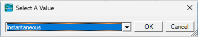
2. Select the Options Button on the Modeling Approach column and select Set:
   
3. Choose Instantaneous: 
   
4. Next open the Node Attribute Table and the Base Area for Node DMH-5 to 50.24 sqft. This is the receiving node for the instantaneous flows and adding the upstream (instantaneous) manholes size to it will increase the computational cell's volume and increase it's stability in receiving the instantaneous flows. 

Set Mesh Cell Length

HEC-RAS will make an initial estimate of a Mesh Cell Length based on the size of the conduit. However, this typically will need adjustment to better stability and faster runtimes. Generally, steeper sloped conduits (like in this dataset) will require smaller cell sizes to better capture the hydraulics and shallower larger conduits can get away with much larger cell sizes. Finding the an acceptable cell size is usually an iterative approach that requires watching for instabilities, and observing the courant values and computation timesteps. 

1. In an Edit Session, Open the Conduit Attribute Table and Sort by Slope, Descending. 
   
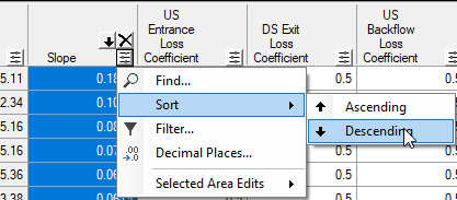
2. Copy - Paste the Cell Size column below into the Conduit Attribute Table using Ctrl+C, Ctrl+V. Note, you may have to bring the values into Excel before pasting them into the Conduits Table.   

   Conduit Name	Slope	Cell Size
   14	0.1886	5
   2	0.108089	10
   6	0.081162	10
   5	0.07871	10
   15	0.065811	10
   13	0.061888	10
   8	0.053077	15
   1	0.036696	15
   12	0.031979	15
   10	0.023447	20
   9	0.021486	20
   7	0.017477	20
   3	0.015788	25
   16	0.015661	25
   11	0.014789	25
   4	0.014779	25

3. Save Edits and Close the Attribute Table.

Setup Boundary Conditions

The Pipe Network in this model will receive inflows exclusively from Drop Inlets connected to the 2D Area. However, the outfall node of the Pipe Network, where the system daylights and flows into Beaver Lake, is an External type node and therefor needs an external boundary condition defined for it. The node is an External type because it is outside of the 2D Area extent and it is above the terrain. To learn more, see the Node Types section of the Pipe Network Geometry User's Manual.

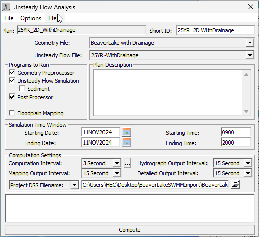
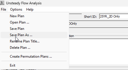
1. From the Unsteady Flow Analysis Window, select File > Save As. Name the new Plan 25YR_2D_With Drainage.
   
2. Set the Geometry File to the Beaver Lake With Drainage geometry and Save the Plan.
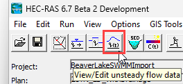
3. Open the Unsteady Flow Data window
   
4. Select File >Save As and provide the new name: 25YR-WithDrainage
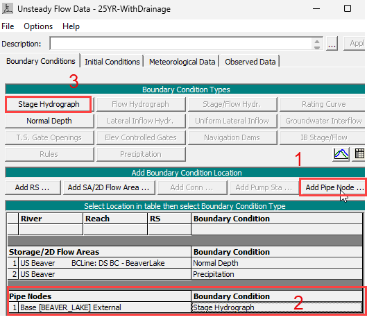
5. Select Add Pipe Node... and select BEAVER LAKE External Node.
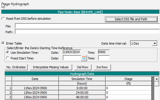
6. Assign the Node a Stage Hydrograph boundary condition.
   
   This Stage Hydrograph would typically represent the receiving lake level or tide level for coastal watersheds. In this case we are not concerned with the lake level so we will set stage to 0 for the whole simulation, representing a free outfall.
   
   

   Free Outfalls on External Nodes

   Modeling a free outfall for an External node Pipe Network can be done by assigning a Stage Hydrograph boundary condition, and setting the stage below the node invert. This will result in plunging flow out of the system and the stage in the conduit will be computed as described in the Hydraulic Reference Manual. 

7. In the Stage Hydrograph editor set the Data Interval to 1 Day. Then fill in a few 0s for the stage. This will ensure a plunging outfall. 
   
8. Save the Unsteady Flow Data.
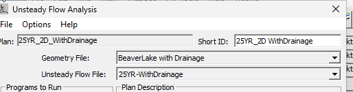
9. Back in the Unsteady Flow Analysis Window, reopen the 25YR_2D_WithDrainage plan and set the Unsteady Flow File to the 25YR-WithDrainage.
10. Save the Plan The plan should look like below:
    
11. Under the Options menu in the Unsteady Flow Analysis Window, select Compute Options.
12. Under the Pipe Network Tab, ensure that Diffusion Wave is the selected, equation set and that the Compute Every 2D Iteration option is On.
    The Compute Every 2D Iteration will solve the Pipe Network each time the 2D area iterates. This option slows down compute performance, but improves stability particularly where Pipe Networks are used to represent culverts. 
    
13. Save the Plan and Select Compute.

Reviewing Results

After the model simulation is complete, we will visualize the results in a few different ways including Pipe Network Profile plots, Stage and Flow Hydrographs and spatial results in HEC-RAS Mapper. 

Profile Plot Results and Spatial Results

1. In HEC-RAS Mapper find the 25YR_2D_WithDrainage Result in the tree. 
2. Right-Click the result and select Plot Results Profile. This will bring up the Pipe Network Profile Plot by default. 
   
3. In the Profile Plot, display all the conduits by clicking in the table in left pane and pressing Ctrl+A.
   
4. Animate the results with the scrubber bar at the top of the window.
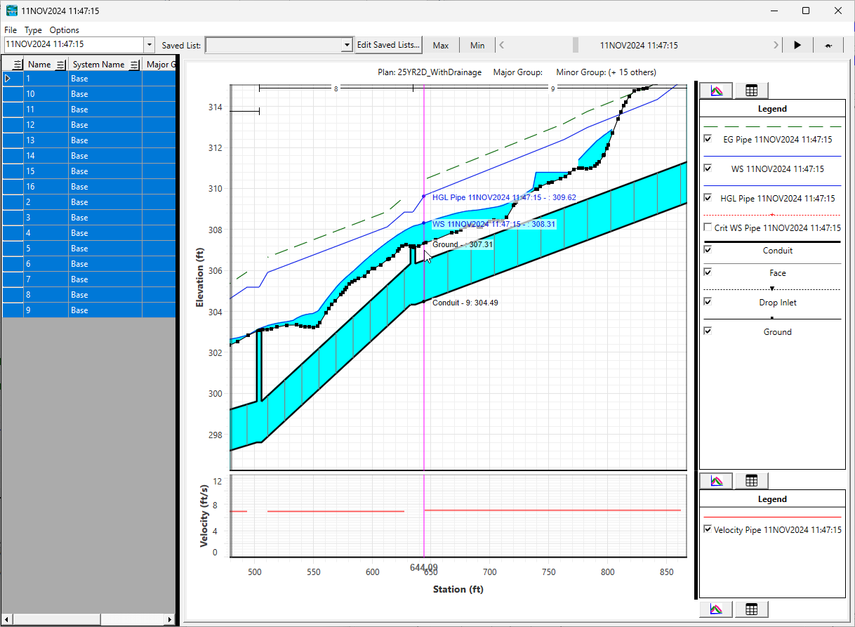
   1. The profile plot displays the Hydraulic Grade Line, Energy Grade Line, and Critical Depth for the Pipe Network, and the water surface elevation for the surface model (2D Area in this case).
   2. Below the profile plot you will see a profile of velocity and flow in the Pipe Network.
   3. You can zoom in and out on the plot, and pan around to get a better look at results. To return to the full view you can Right-Click and select Full Plot.

From the Profile Plot you can see the much of the Pipe Network is in supercritical flow early in the simulation which makes sense given the steep slopes of the Pipes. That said, high velocities are expected as well. 

Then, about 1/4 way into the simulation, the system becomes overwhelmed on the downstream end and begins to pressurize the system further upstream. As the system begins surcharging, you can see the velocities in the conduits decrease significantly.

At it's peak the pipe network HGL exceeds both the Drop Inlet elevations and the water surface elevation in the 2D Area above such that water begins flowing from the Pipe Network onto the surface. More on that in the Stage and Flow Hydrograph section next.

Spatial Results for the Pipe Network can also be turned for the Pipe Network such as Pipe WSE (HGL), Pipe Depth, Pipe Velocity, and Pipe Percent Full.

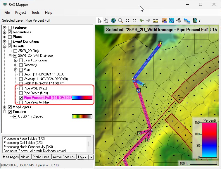
Pipe Rending Options Found under Tools>Options allow for the scaling the of pipe spatial results for easier visualization:

Stage & Flow Hydrograph Results

1. Open the Stage and Flow Hydrograph Plot
   
2. In the Stage and Flow Plot, Select the Type menu and change to Pipe Nodes.
3. Select the INLET-5 Node from the Node dropdown. 
   This is a location where the HGL exceeded the water surface elevation above resulting in flow surcharging from the pipe network on to the surface (shown as negative flow). The inflow or outflow at Drop Inlets is computed based on a family of rating curves that take into account the head differential between the surface and the Pipe Network stages. For more information on that see the Hydraulic Reference Manual for Pipes.
   Figure: Inlet 5 Flow Hydrograph Surcharging

   

4. Next select the BEAVER_LAKE node. This is the outfall for the system and you can see the the peak flows are over 50 CFS.

Conclusion

This tutorial demonstrated how to import Pipe Network geometry into HEC-RAS from an existing EPA SWMM model, setup model boundary conditions, setup a simulation and review basic results. We started with a 2D rain-on-mesh model, added a pipe network and connected the pipe network to the surface model at several Drop Inlets and a Culvert Opening type node.

To continue learning how to model Pipe Networks in HEC-RAS with this dataset you can try adding additional Pipe Networks using the hand editing tools to drain other portions of the model. Another continuation is to try increasing the size of the existing pipe Network, or add parallel conduits to prevent surcharging.