Download PDF
Download page HEC-RAS 2D Modeling Advantages/Capabilities.
HEC-RAS 2D Modeling Advantages/Capabilities
The 2D flow routing capabilities in HEC-RAS have been developed to allow the user to perform 2D or combined 1D/2D modeling. The 2D flow modeling algorithm in HEC-RAS has the following capabilities:
- Can perform 1D, 2D, and combined 1D and 2D modeling. HEC-RAS can perform 1D modeling, 2D modeling (no 1D elements), and combined 1D and 2D modeling. The ability to perform combined 1D/2D modeling within the same unsteady flow model will allow users to work on larger river systems, utilizing 1D modeling where appropriate (for example: the main river system), and 2D modeling in areas that require a higher level of hydrodynamic fidelity.
- Shallow Water Equations (SWE) or Diffusion Wave Equations (DWE) in 2D. The program solves either the 2D Shallow Water equations (with optional momentum additions for turbulence, wind forces, mud and debris flows, and Coriolis effects) or the 2D Diffusion Wave equations. This is user selectable, giving modelers more flexibility. In general, the 2D Diffusion Wave equations allow the software to run faster and have greater stability properties. The 2D Shallow Water equations are applicable to a wider range of problems. However, many modeling situations can be accurately modeled with the 2D Diffusion Wave equations. Because users can easily switch between equation sets, each can be tried for any given problem to see if the use of the 2D Shallow Water equations is warranted over the Diffusion Wave equations.
- Implicit Finite Volume Solution Algorithm. The 2D unsteady flow equations solver uses an Implicit Finite Volume algorithm. The implicit solution algorithm allows for larger computational time steps than explicit methods. The Finite Volume Method provides an increment of improved stability and robustness over traditional finite difference and finite element techniques. The wetting and drying of 2D cells is very robust. 2D flow areas can start completely dry, and handle a sudden rush of water into the area. Additionally, the algorithm can handle subcritical, supercritical, and mixed flow regimes (flow passing through critical depth, such as a hydraulic jump) without any special options to turn on.
- 1D and 2D Coupled Solution Algorithm. The 1D and 2D solution algorithms are tightly coupled on a time step by time step basis with an option to iterate between 1D and 2D flow transfers within a time step. This allows for direct feedback each time step between the 1D and 2D flow elements. For example, consider a river that is modeled in 1D with the area behind a levee is modeled in 2D (connected hydraulically with a Lateral Structure). Flow over the levee (Lateral Structure) and/or through any levee breach is computed with a headwater from the 1D river and a tailwater from the 2D flow area to which it is connected. The weir equation is used to compute flow over the levee and through the breach. Each time step the weir equation uses the 1D and the 2D results to compute the flow allowing for accurate accounting of weir submergence, at each time step, as the interior area fills up. Additionally, flow can go back out of the breach (from the 2D area to the 1D reach), once the river stages subside.
- Unstructured or Structured Computational Meshes. The software was designed to use unstructured computational meshes but can also handle structured meshes. A structured mesh is treated the same as an unstructured mesh. The software assumes that cells are orthogonal to each other (the face between two cells is perpendicular to a line connecting the two cell centers). Assuming orthogonality simplifies some of the computations required and improves computational speed. This means that computational cells can be triangles, squares, rectangles, or even five and six-sided elements (the model is limited to elements with up to eight sides). The mesh can be a mixture of cell shapes and sizes. The outer boundary of the computational mesh is defined with a polygon. The computational cells that form the outer boundary of the mesh can have very detailed multi-point lines that represent the outer face(s) of each cell.
- Detailed Hydraulic Property Tables for 2D Computational Cells and Cell Faces. Within HEC-RAS, computational cells do not have to have a flat bottom, and cell faces/edges do not have to be a straight line, with a single elevation. Instead, each Computational cell and cell face is based on the details of the underlying terrain. This type of model is often referred to in the literature as a "high resolution subgrid model" (Casulli, 2008). The term "subgrid" means it uses the detailed underlying terrain (subgrid) to develop the geometric and hydraulic property tables that represent the cells and the cell faces. HEC-RAS has a 2D flow area pre-processor that processes the cells and cell faces into detailed hydraulic property tables based on the underlying terrain used in the modeling process. For an example, consider a model built from a detailed terrain model (2ft grid-cell resolution) with a computation cell size of 200x200 ft. The 2D flow area pre-processor computes an elevation-volume relationship, based on the detailed terrain data (2ft grid), within each cell. Therefore, a cell can be partially wet with the correct water volume for the given water surface elevation (WSEL) based on the 2ft grid data. Additionally, each computational cell face is evaluated similar to a cross section and is pre-processed into detailed hydraulic property tables (elevation versus - wetted perimeter, area, roughness, etc…). The flow moving across the face (between cells) is based on this detailed data. This allows the modeler to use larger computational cells, without losing too much of the details of the underlying terrain that govern the movement of the flow. Additionally, the placement of cell faces along the top of controlling terrain features (roads, high ground, walls, etc…) can further improve the hydraulic calculations using fewer cells overall. The net effect of larger cells is fewer computations, which means much faster run times. An example computational mesh overlaid on detailed terrain is illustrated in Figure 1-1.

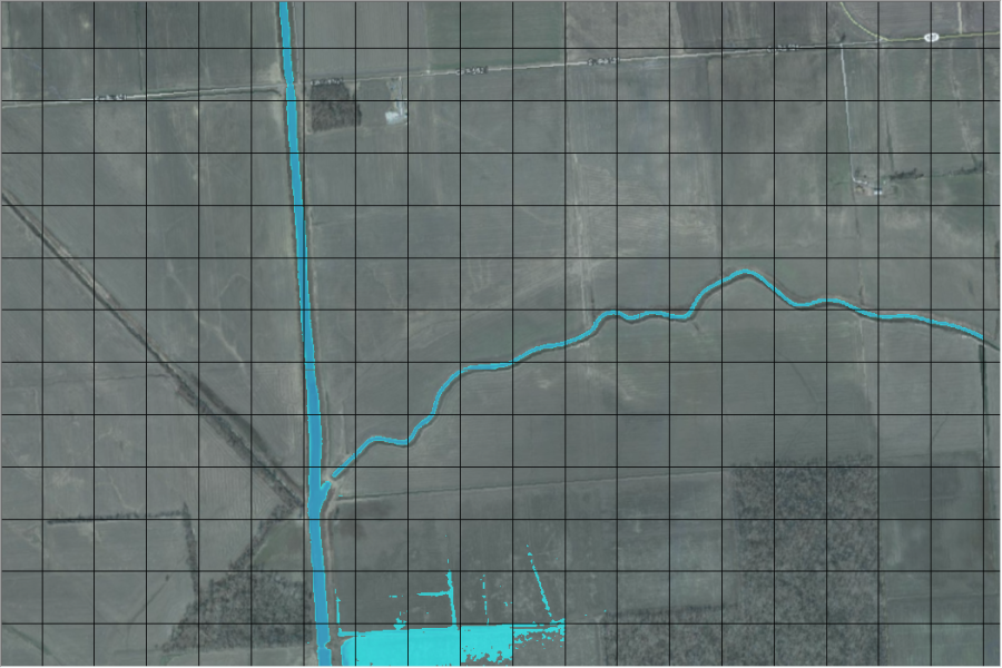
Shown in Figure 1-1 is an example computational mesh over terrain data depicted with color shaded elevations. The computational cells are represented by the thick black lines. The cell computational centers are represented by the black dots and are the locations where the water surface elevation is computed for each cell. The elevation-volume relationship for each cell is based on the details of the underlying terrain. Each cell face is a detailed cross section based on the underlying terrain below the line that represents the cell face. This process allows for water to move between cells based on the details of the underlying terrain, as it is represented by the cell faces and the volume contained within that cell. Therefore, a small channel that cuts through a cell, and is much smaller than the cell size, is still represented by the cell's elevation volume relationship, and the hydraulic properties of the cell faces. This means water can run through larger cells, but still be represented with its normal channel properties. An example of a small channel running through much larger grid cells is shown in Figure 1-2. The example shown in Figure 1-2 has several canals that are much smaller than the average cell size used to model the area (cell size was 500 x 500 ft, where the canals are less than 100 ft wide). However, as shown in Figure 1-2, flow is able to travel through the smaller canals based on the canal's hydraulic properties. Flow remains in the canals until the stage is higher than the bank elevation of the canal, then it spills out into the overbank areas.
- Detailed Flood Mapping and Flood Animations. Mapping of the inundated area, as well as animations of the flooding can be done inside of HEC-RAS using the RAS Mapper features. The mapping of the 2D flow areas is based on the detailed underlying terrain. This means that the wetted area will be based on the details of the underlying terrain, and not the computational mesh cell size. Computationally, cells can be partially wet/dry (this is how they are computed in the computational algorithm). Mapping of the results will reflect those details, rather than being limited to showing a computational cell as either all wet or all dry.
- Multi-Processor Based Solution Algorithm (Parallel Computing). The 2D flow area computational solution has been programmed to take advantage of multiple processors on a computer (referred to as parallelization), allowing it to run much faster than on a single processor.
- 64-Bit Computational Engines. HEC-RAS now comes with 64-bit computational engines. The 64-bit computational engines run faster than the previous 32-bit and can handle much larger data sets. 32-bit computations are no longer supported, and user's must be running a 64-bit operating system.