Download PDF
Download page Development of the 2D Computational Mesh.
Development of the 2D Computational Mesh
The HEC-RAS 2D modeling capability uses a Finite-Volume solution scheme. This algorithm was developed to allow for the use of a structured or unstructured computational mesh. This means that the computational mesh can be a mixture of 3-sided, 4-sided, 5-sided, etc… computational cells (HEC-RAS has a maximum of 8 sides in a computational cell). However, users typically select a nominal grid resolution to use (e.g., 200 ft x 200 ft cells), and the automated tools within HEC-RAS will build the computational mesh. After the initial mesh is built, the user can refine the grid with break lines, refinement regions, and the mesh editing tools. A 2D computational mesh is developed in HEC-RAS Mapper by doing the following:
Drawing a Polygon Boundary for the 2D Area
The user must add a 2D flow area polygon to represent the boundary of the 2D area using the geometry editing tools in HEC-RAS Mapper. The best way to do this in HEC-RAS is to first bring in terrain data and aerial imagery into HEC-RAS Mapper. Additionally, the user may want to bring in a shapefile that represents a protected area, if they are working with a leveed system. The terrain and background images will assist the user in figuring out where to draw the 2D flow area boundaries.
To create the 2D flow area in HEC-RAS Mapper, do the following: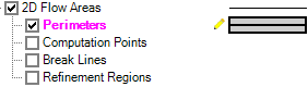
1. Right click on the Geometry Layer to edit, and select Edit Geometry.
2. Expand the 2D Flow Areas layer and select the Perimeters layer.
3. Draw the perimeter using the Add New Feature ![]() tool.
tool.
Zoom in to the point at which you can see with great detail, where to draw the boundary of the 2D Flow Area. Begin by left clicking to drop a point along the 2D flow area polygon boundary. Then continue to use the left mouse button to drop points in the 2D flow area boundary. As the user runs out of screen real-estate, they can right click to re-center the screen, this will give you more area to continue drawing the 2D flow area boundary. Double click the left mouse button to finish creating the polygon. Once the 2D area polygon is finished, the interface will ask the user for a Name to identify the 2D flow area. Shown in Figure 3-1 is an example 2D flow area polygon for an area that is protected by a levee. The name given to the 2D flow area in this example is: “2D Interior Area”.

Create the 2D Computational Mesh
The HEC-RAS terminology for describing the computational mesh for 2D modeling begins with the 2D flow area. The 2D flow area defines the boundary for which 2D computations will occur. A computational mesh (or computational grid) is created within the 2D flow area. Each cell within the computational mesh has the following three properties (Figure 3-2).
Cell Center:The computational center of the cell. This is where the water surface elevation is computed for the cell. The cell center does not necessarily correspond to the exact cell centroid.
Cell Faces:These are the cell boundary faces. Faces are generally straight lines, but they can also be multi-point lines, such as the outer boundary of the 2D flow area.
Cell Face Points:The cell Face Points (FP) are the ends of the cell faces. The Face Point (FP) numbers for the outer boundary of the 2D flow area are used to hook the 2D flow area to a 1D elements and boundary conditions.
After the 2D Flow Area polygon boundary is created, the next step is to begin creating the computational mesh. In general, the user should decide on a base cell size to use for the 2D flow area. Keep in mind that you will be able to refine the mesh with breaklines and refinement regions where needed. To create the base mesh, do the following:
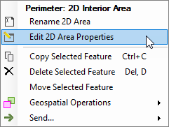
1. Select the 2D Flow Area polygon to be edited.
2. Right click on the 2D Flow Area and select Edit 2D Area Properties.
3. Once that menu option is selected a window will appear as shown in Figure 3-3 below. 
4. In the Computational Points portion of the editor, enter the Points Spacing DX and DY values. Press the Generate Computation Points with All Breaklines button to generate the base mesh. Pressing this button will cause the software to compute a series of X and Y coordinates for the cell centers. The user can view these points by pressing the View/Edit Computational Point's button ![]() , which brings the points up in a table. The user can cut and paste these into a spreadsheet or edit them directly if desired (It is not envisioned that anyone will edit the points in this table or Excel, but the option is available).
, which brings the points up in a table. The user can cut and paste these into a spreadsheet or edit them directly if desired (It is not envisioned that anyone will edit the points in this table or Excel, but the option is available).
5. If you want to have a default Manning's n value for the 2D Flow Area, it can be entered under the Hydraulic Cell/Face Properties area of the editor. The Default Manning's n Value will be used for the cell faces in the 2D flow area. Users have the option of adding a spatially varying Land Use classification versus Manning's n value table (and a corresponding Land Classification layer in RAS-Mapper), which can be used to override the base Manning's n values where polygons and roughness are defined. Even if a Land Use Classification versus Manning's n value table is defined, for any areas of the 2D flow area not covered by that layer, the base/default Manning's n value will be used for that portion of the 2D flow area.
Additionally, there is a gear button ![]() that can be used to bring up an editor that allows the user to change the tolerances used when creating the hydraulic property tables for the 2D cells and faces. The following is a description of these tolerances:
that can be used to bring up an editor that allows the user to change the tolerances used when creating the hydraulic property tables for the 2D cells and faces. The following is a description of these tolerances:
- Cell Elev-Vol Filter Tol: This tolerance is used to reduce the number of points in the 2D cell elevation volume curves that get developed in the 2D pre-processor. Fewer points in the curve will speed up the computations but reduce the accuracy of the elevation volume relationship. The default tolerance for filtering these points is 0.01 ft.
- Cell Minimum Area Fraction: This field is used to enter a fraction that is multiplied by the cell area to establish a minimum area at the lowest elevation of the cell. The purpose of this field is to prevent the cell elevation volume curves from going down to an extremely small area at the bottom of the cell, and then creating a curve that is very abrupt at the lowest end. Establishing a reasonable minimum area for the cell helps out with the stability of solving that cell when it first starts to get water. The default is 0.01 (1 %).
- Face Profile Filter Tol: This filter tolerance is used to reduce the number of points that get extracted from the detailed terrain for each face of a 2D cell. The default is 0.01 ft.
- Face Area-Elev Filter Tol: This filter tolerance is used to reduce the number of points in the cell face hydraulic property tables. Fewer points in the curves will speed up the computations but reduce the accuracy of the face hydraulic property relationships. The default is 0.01 ft.
- Face Conveyance Tol Ratio: This tolerance is used to figure out if more or less points are required at the lower end of the face property tables. It first computes conveyance at all of the elevations in the face property tables. It then computes the conveyance at an elevation half way between the points and compares this value to that obtained by using linear interpolation (based on the original points). If the computed value produces a conveyance that is within 2% (0.02) of the linear interpolation value, then no further points are needed between those two values. If linear interpolation would produce a value of conveyance that is more than 2% from the computed value at that elevation, then a new point is added to that table. This reduces the error in computing hydraulic properties, and therefore conveyance due to linear interpolation of the curves. A higher tolerance will result in fewer points in the hydraulic property tables of the cell faces, but less hydraulic accuracy for the flow movement across the faces. The default value is 0.02, which represents a 2% change.
- Face Laminar Depth (ft): At very shallow depths on planar surface (e.g. A parking lot or a road) the flow can be laminar instead of turbulent. If the flow is assumed to be turbulent all the way to a zero depth, then the program will underestimate the velocity of flows down a plane at very shallow depths. This field is used as the transition point from turbulent to laminar flows. Anything below this depth will assumed to be laminar flow and treaded as such.
6. You have the option to run the 2D Flow Area pre-processor right from this editor if you want to. This is accomplished by pressing the Compute Property Tables button. This step is not necessary, until the mesh is further refined, and you plan on performing a computation. The 2D pre-processor will automatically run when the user performs a Compute if the tables are out of date.
7. Press the Close button to close the editor and accept the mesh and property settings. An example of a base mesh, with not break lines or refinement regions, is shown in Figure 3-4.

Editing/Modifying the Computational Mesh.
The computational mesh will control the movement of water through the 2D flow area. Specifically, one water surface elevation is calculated for each grid cell center at each time step. The computational cell faces control the flow movement from cell to cell. Within HEC-RAS, the underlying terrain and the computational mesh are preprocessed in order to develop detailed elevation–volume relationships for each cell, and detailed hydraulic property curves for each cell face (elevation vs. wetted perimeter, area, and roughness). By creating hydraulic parameter tables from the underlying terrain, the net effect is that the details of the underlying terrain are still considered in the water storage and conveyance, regardless of the computational cell size. However, there are still limits to what cell size should be used, and important considerations for where smaller detailed cells are needed versus larger coarser cells.
In general, the cell size should be based on the slope of the water surface in a given area, as well as barriers to flow within the terrain. Where the water surface slope is flat and not changing rapidly, larger grid cell sizes are appropriate. Steeper slopes, and localized areas where the water surface elevation and slope change more rapidly will require smaller grid cells to capture those changes. Since flow movement is controlled by the computational cell faces, smaller cells may be required to define significant changes to geometry and rapid changes in flow dynamics.
HEC-RAS makes the computational mesh by following the Delaunay Triangulation technique and then constructing a Voronoi diagram (see Figure 3-5 below, taken from the Wikimedia Commons, a freely licensed media file repository):
The triangles (black) shown in Figure 3-5 are made by using the Delaunay triangulation technique (http://en.wikipedia.org/wiki/Delaunay_triangulation ). The cells (red) are then made by bisecting all of the triangle edges (black edges), and then connecting the intersection of the red lines (Voronoi diagram). This is analogous to the Thiessen Polygon method for attributing basin area to a specific rain gage.
The computational mesh can be edited/modified with the following tools: break lines; refinement regions; moving points; adding points, and deleting points.
Break Lines
Either before or after the computational mesh is created the user may want to add break lines to force the mesh to align the computational cell faces along the break lines. In general, break lines should be added to any location that is a barrier to flow, or controls flow/direction. The user should align the faces of the 2D mesh for areas that are barriers to flow in order to accurately capture the high ground with cell faces. Examples where this should always be done are levees, roads, and natural berms in the terrain.
The user can add new break lines at any time. HEC-RAS allows the user to enter a new break line on top of an existing mesh and then regenerate the mesh around that break line, without changing the computational points of the mesh in other areas. Break lines can be drawn by hand; imported from Shapefiles; or detailed coordinates for an existing break line can be pasted into the break line coordinates table.
To add break lines by hand into a 2D flow area (while in the geometry editing mode), select the Break Lines layer (it should then be highlighted in magenta), then left click on the location within the 2D flow area that you want to start a break line. Left click to add additional points, and right click to re-center the view within the window. Double click to end a break line. Once a break line is drawn the software will ask you to enter a name for the break line. After the break line is entered, the mesh generation tools will automatically try to "snap" the cell faces to the break lines. The cells formed around break lines may not always have cell faces that are aligned perfectly with the break lines. The user can draw a new break line, then right click on the break line and select the option Enforce Break line. Once this option is selected, new cells will be generated around the break line with cell faces that are aligned along the break line. Any existing cell centers that were already in the mesh in the area of the break line are remove first (within a buffer zone around the break line, based on the cell size used around the break line). By default, the cell size used along the break line will be equal to the nominal cell size entered for the 2D flow area.
Additionally, the user can control the size/spacing of cells along the break line. When creating a mesh around a break line, it may be desirable or even necessary to use smaller cells than the nominal cell size used in other areas of the mesh. To control the cell spacing along a break line, right click on the Break Lines layer and select the option Open Attribute Table (Figure 3-6). A window will appear allowing the user to enter: a Near Spacing; Near Repeats; and a Far Spacing. There is also an option to "Enforce a 1 Cell Protection Radius" around the break line. This option protects the cells immediately around the break line from being deleted or moved due to other break lines that may be very close. The Near Spacing field is used to enter the cell size you want right along the break line. The Near Repeats field is an optional field that allows you to repeat the cell size define in the Near Spacing filed multiple times. For example, if the user entered a Near Spacing of 50 ft, then the cells on both sides of the break line would be 50 ft cells. If the user also entered a Near Repeats of 2, then two additional rows of 50 ft cells would be placed on both sides of the break line. The Far Spacing option allows the user to control how far the software will increase the cell size as it gradually transitions from the Near spacing to the user entered Far Spacing. If a Far Spacing is not entered, it is automatically set to the nominal cell size of the 2D flow area. The software will then increase the cell size around the break line, in order to provide a gradual cell size transition from the break line to the Far Spacing cell size being used for the mesh.

To import Break lines from a shapefile, while editing the break lines, right click on the Break Lines layer and select Open Attribute Table. At the lower right hand corner of this editor is a button labeled Import Features (Figure 3-6). Select the Import Features button and a file browser will come up. Find the Shapefile that contains the lines that you want to use as break lines and select that file. Then press the Open button.
An example of using break lines within a 2D flow area for modeling levees and roads is shown in Figure 3-7.

Mesh Refinement Regions
Refinement regions are a mesh editing tool that allows the user to refine or coarsen an area of the mesh. A polygon is created to define the boundary of the refinement area. The interior of the area is given a cell spacing (just like the Perimeter layer) and the bounding polyline is given a point spacing (just like a break line). Refinement regions can be used to densify an area where more detailed results are desired due to rapid changes in terrain or water surface elevation, or to simplify an area where the water surface elevation will not vary much and users want to reduce the number of computation points in the 2D Flow Area.
Additionally, refinement regions can also be used to create a good mesh in the main channel regions of the model. To add a refinement region, do the following:
1. While editing the geometry in HEC-RAS Mapper, select the refinement region layer. It should turn to a magenta color if it is selected.
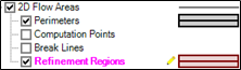
2. Select the Add New Feature editing tool, then left click to start drawing the refinement region polygon. Continue to left click to add additional vertices to the polygon. As you are drawing the polygon, users can right click to re-center the drawing window. Double click to end the refinement region polygon. A window will pop up asking the user to enter a name for the refinement region.
Additional properties for controlling how the refinement regions affect the 2D Flow Areas are accessed through the Refinement Region Editor. This editor is available by right clicking on the feature or the Refinement Region layer and selecting the Edit Refinement Region Properties shortcut menu item. The Refinement Region Editor allows users to modify the properties of each region.
When a refinement polygon is enforced, the boundary is treated much like a break line, where the point spacing along the break line grows larger farther away from the line. This transition of cell sizes happens both outside of the boundary and on the inside of the polygon. As shown in Figure 3-8, the properties for each refinement area include the Name, Cell Spacing X, Cell Spacing Y, Perimeter Spacing, Near Repeats, and Far Spacing. These properties (described below) control how the refinement region will be used to modify the mesh, when enforced (e.g., Figure 3-8).

.
- Name – Each region must have a unique name and the editor.
- Cell Spacing X – The spacing distance in the X-direction for adding computation points inside of the refinement region.
- Cell Spacing Y – [NOT IMPLEMENTED YET] The spacing distance in the Y-direction for adding computation points inside of the refinement region.
- Perimeter Spacing – The distance to add computation points along the region boundary (i.e., how often points are added) just as done with the Near Spacing on the Breakline layer. The points are generally placed along the line offset by ½ of the spacing value. If not specified, the default value is the Cell Spacing X value.
- Near Repeats – The number of times to duplicate the Perimeter Spacing on both sides of the perimeter before transitioning to the Far Spacing. If not specified, the default value is zero.
- Far Spacing – How large a distance to go when adding points away from the line. Computation points will be added sequentially starting with the Near Spacing and doubling the previous spacing until the Far Spacing values is achieved (approximately). If not specified, the default value is the point spacing on the 2D Flow Area.
- Enforce 1 Cell Protection Radius – A protective region buffered around the perimeter that extends by the Perimeter Spacing distance on each side. Within this protection region, cells can neither be added nor removed by the cell generation routines. This means that any previous hand-edits to those cells will remain, and any nearby break lines cannot interfere with this already-enforced region.
A simple example of using two refinement regions to simplify and densify a mesh are shown in Figure 3-9.
Making a Channel Mesh
Another use for the refinement region is around the main channel of a stream. Shown in Figure 3-10 is an example where a single refinement region was created for the entire main channel. By doing this, the user can control the cell size inside of the channel and ensure that cell faces are aligned with the high ground at the main channel banks. This approach ensure that flow does not spill out of the channel until the water is high enough to cross over the outer cell faces representing the high ground of the main channel bank lines. In addition to the refinement region, a break line was placed right down the center of the refinement region, following the path of the flow. The break line is used to align the cells in the middle of the channel with the direction of the flow. For the breakline in the example below, the number of near repeats was set to 4. For the refinement region, the near repeats was set to zero. Additionally, the option to "Enforce a 1 cell protection radius" was turned on for both the refinement region and the break line. Also, the break line was enforced after the refinement region. This combination of a refinement region and a break line down the center of the channel makes for a very nice channel mesh (Figure 3-10).

Hand Based Mesh Editing Tools
The hand editing mesh manipulation tools are available under the Edit menu of the HEC-RAS Geometric Data editor and are also available in HEC-RAS Mapper. From the Geometric editor, if the user selects Edit then Move Points/Object, the user can select and move any cell center or points in the bounding polygon. If a cell center is moved, all of the neighboring cells will automatically change due to this movement. If the user selects Edit then Add Points, then wherever the user left clicks within the 2D flow area, a new cell center is added, and the neighboring cells are changed (once the mesh is updated). The software creates a local mesh (Just the area visible on the screen, plus a buffer zone), such that while you are editing, just the local mesh will get updated. The entire mesh only updates once the user has turned off the editing feature, which saves computational time in creating the new mesh. If the user selects Edit then Remove Points, then any click near a cell center will remove that cell's point, and all the neighboring cells will become larger to account for the removed cell.
From HEC-RAS Mapper, the user can also hand edit the 2D Flow Area boundary and computation points. Start editing the Geometry in HEC-RAS Mapper, then select the Perimeter to edit the boundary, or select Computational Points to edit the cell computational points. To add new cell points, use the Add New Feature editing tool. To move or delete points use the Edit Feature tool.
The user may want to add points and move points in areas where more detail is needed. The user may also want to remove points in areas where less detail is needed. Because cells and cell faces are preprocessed into detailed hydraulic property tables, they represent the full details of the underlying terrain. In general, the user should be able to use larger grid cell sizes than what would be possible with a model that does not preprocess the cells and the cell faces using the underlying terrain. Many 2D models simply use a single flat elevation for the entire cell, and a single flat elevation for each cell face. These types of 2D models generally require very small computational cell sizes in order to model the details of the terrain.
Potential Mesh Generation Problems
The automated mesh generation tool in HEC-RAS works well, however, nothing is perfect. On occasion a bad cell will be created due to the combination of the user defined polygon boundary and the selected nominal cell size, or when the user is adding/modifying points inside of the polygon. After the mesh is made, the software automatically evaluates the mesh to find problem cells. If a problem cell is found, that cell's center is highlighted in a red color, and a red message will show up on the lower left corner of the geometric data window. Here is a list of some problems that are possible, and how to fix them with the mesh editing tools described above:
- Mesh Boundary Issues: When the user draws a 2D flow area boundary that is very sharp and concave, depending on the cell size selected, the mesh generation algorithm may not be able to form a correct mesh at this location (Figure 3-11). To fix this problem, the user can either add more cell centers around the concave portion of the boundary, or they can smooth out the boundary by adding more points to the boundary line, or both.

Shown in Figure 3-12 is the fixed mesh. The mesh was fixed by smoothing out the sharp concave boundary and adding some additional cell centers around the sharp portion of the boundary.

- Too Many Faces (sides) on a Cell: Each cell is limited to having 8 faces (sides). The HEC-RAS mesh development routines check for cells with more than 8 sides. If a cell exists with more than 8 sides it will be highlighted in red and a message will appear in the lower left portion of the geometric data window. An example of a cell with more than 8 sides is shown in Figure 3-13. If you have a cell with more than 8 sides you will need to edit that cell and/or the cells that bound it. Use the tools found in the Geometric editor under the "Edit" Menu. Available tools are (1). Add Points: to add points to the cell boundary polygon, or additional cells; (2). Remove Points: to delete points in the boundary polygon or delete cells; and (3). Move Points/Objects: to move the boundary points or the cell centers.

The mesh problem shown in Figure 3-13 (cell with more than 8 sides) was fixed by adding additional cell centers in the area of this cell, which made the cell size smaller and reduced the number of sides of the cells. The fixed mesh is shown in Figure 3-14.

- Duplicate Cell Centers: If a user accidentally puts a point right on top of, or very close to an existing cell center, this will cause a mesh generation problem. The mesh generation tools search for this issue and will identify any cell with duplicate cell centers. The solution to this problem is to delete one of the cell centers.
- Cell Centers Outside of the 2D flow area Polygon. If a user accidentally drops a point outside of the 2D flow area polygon, or they move the polygon boundary to the point in which cell centers are outside the polygon, this will generate a mesh error. The mesh routines will identify any points that are outside the current boundary. To fix the mesh, simply delete the points that are outside of the 2D flow area boundary.
- Cells with Collinear Faces (Break Lines too close together). Computational cells used within the HEC-RAS 2D code cannot have two faces that are collinear (i.e., they cannot form a straight line). Where two cells meet (at a face point), the outside angle formed by the two faces must be greater than 180 degrees. This is called "Strict Convex" in mathematical terms. Meaning all cells are require to be strictly convex, and therefore no two faces within the same cell can be collinear (Form a straight line). If cells end up like this, the software will run, but the computation across cell faces that are like this will not be correct.
This problem is generally caused by placing two or more break lines parallel to each other, and close together, such that the creation of cells along one break line can create problems with cells along the other break line. Cells are created along break lines one at a time. Additionally, the user can specify a cell min and max size to form the cells around a break line. The min cell size gets used right along the break line, then it transitions out the max cell size by doubling the cell size as it goes outward from the break line. If the user does not put in a max cell size, the software assumes that they want to transition out to the nominal cell size that was entered in the 2D Flow Area editor.
If the break lines are close together, this transitioning out can "Bleed" over into the cell space along a neighboring break line. This can have the effect of forming cells that no longer follow the first break line, but even worse, cells could be formed that are not correct/consistent with the HEC-RAS 2D solution scheme. Below (Figure 3-15) is an example in which break lines were used for the channel bank lines and the channel centerline. In this case, all break lines were being transition out to the maximum cell size, which caused this bleed over effect. In this example the channel centerline break line was enforced first, then the channel bank lines. The cells around the channel bank lines were formed correctly, but the cells along the channel centerline were not, due to the fact that the cells formed from the channel bank line break lines override the previously formed cells along the channel centerline (Simply because the order in which they were enforced).
To fix this issue, you can either enter a max cell size that prevents that break lines cells from bleeding over into the neighboring break line cells, or you can enforce the break lines by hand, thus controlling the order in which cells get formed. This specific example was fixed by enforcing the Channel centerline by hand as the last break line to be enforced. See the fixed mesh in Figure 3-16.

