Introduction

In HEC-RAS Versions 6.2 and earlier, the water level (i.e. stage) boundary condition can only be specified as single time-series per boundary condition line. In other words, the water level is spatially constant along the boundary condition line. In HEC-RAS 6.3, the option was added to specify a spatially variable water level boundary condition. This option is especially useful for nesting HEC-RAS within other models, such as ADCIRC. In this new feature, the user can specify any number of time series along a boundary condition line. The location of each water level time series is specified as a fractional distance along the boundary condition line. Open-source and prebuilt binary utilities have been developed which make it easier for users to extract water level time series along HEC-RAS boundaries. These utilities are described in subsequent sections and are provided to users so that they can be run on different platforms and operating systems. The utilities for interpolating water levels are specific to the ADCIRC model but the other models can be used if their output is converted to the ADCIRC format. The method for specifying the water levels along boundary condition lines is quite general and is not model specific. 

Interpolating Water Level Time-Series from ADCIRC Solutions

For most practical applications, ADCIRC is run on very large computational domains for many events producing large computational meshes and solution files. In addition, ADCIRC is typically run on High-Performance Computers (HPC) which utilize a Linux type operating system while HEC-RAS is always run on desktop Windows computers. These factors complicate the extraction of HEC-RAS water level boundary conditions. With the utilities provided, it is possible to extract water level time series directly from the full domain ADCIRC simulations and then transfer the water level time series files from the HPC onto the computers running HEC-RAS. The disadvantage of this approach is that if the HEC-RAS boundary condition line or mesh are modified the user may need to repeat this step and transfer the water level time series files again from the HPC. An alternative approach is to extract water levels on an ADCIRC subdomain encompassing the HEC-RAS boundaries, transfer these files from the HPC, and then extract boundary water levels on the Windows desktop from the subdomain water level solution files.

Creating a Boundary Coordinates File

The Boundary Coordinates File is a simple Comma Separated File (CSV) which contains the WGS84 coordinates of the boundary faces. The coordinates are used to interpolate water levels from ADCIRC simulation results. ADCIRC meshes are typically in Geospatial Coordinates while HEC-RAS projects are always in Projected Coordinates such as State Plane or UTM. The coordinates of the boundary faces can be viewed in the Geospatial Coordinate system WGS84 by right-clicking on the boundary and selecting View WGS84 Coordinates of Faces ... from the menu as shown in the figure below. 

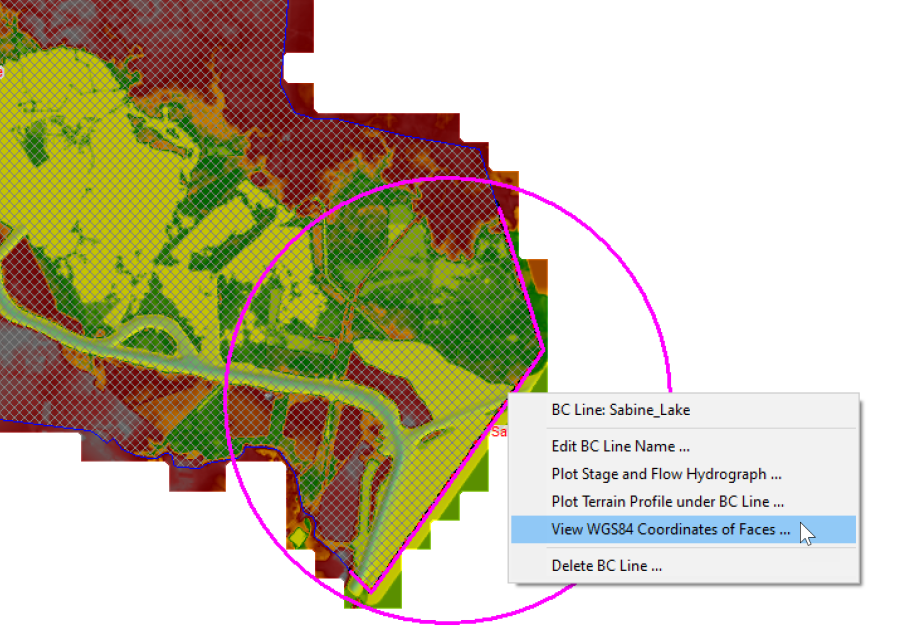Figure 1. Menu to View WGS84 Coordinates of Faces.

HEC-RAS displays both the Projected and Geospatial (i.e. Longitude and Latitude) coordinates of the boundary face centers as shown in the figure below. 

Figure 2. HEC-RAS boundary condition face coordinates in both Projected and WGS84.

The columns for the Longitude and Latitude can be copy-pasted into a Boundary Coordinates File CSV file like the example shown in the figure below. The columns correspond to the Longitude and Latitude, respectively, of the boundary face center coordinates. 

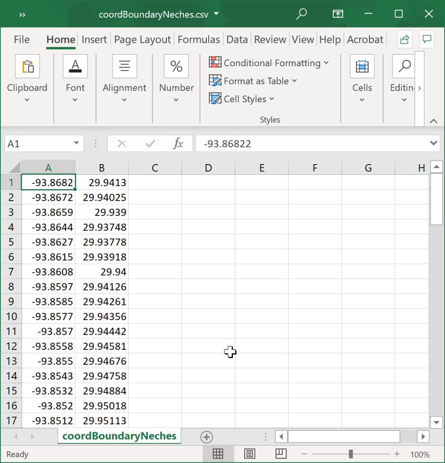
Figure 3. Boundary Coordinates CSV File.

Interpolating Water Level Time-Series at Boundary Condition Points from a Full ADCIRC Domain

The most direct way of obtaining water level time-series for a HEC-RAS boundary condition, is to directly interpolate the water-levels from a full ADCIRC domain. This can be done by either calling the Nesting.exe utility or by calling the Fortran library. Below are two examples of interpolating water levels from a full ADCIRC domain using the Nesting.exe utility.

>Nesting.exe -interpwse "fort.grd" "coordBoundary.csv" "Run1.63" "Run1.csv"
>Nesting.exe -interpwse "fort.grd" "coordBoundary.csv" "Run1.63" "Run1.csv" "Run2.63" "Run2.csv" > log.txt

In the second example two ADCIRC runs are processed at the same time. Any number of ADCIRC simulations can be processes at the same time this way. It is noted that the output from the Nesting.exe command can be redirected to a log file using the ">" operator followed by the name of the output file. The second example above also shows how to redirect the command standard output to a log file called log.txt. When utilizing the Nesting.exe utility it is important that every file (including the executable) have correct paths if not in the local directly.
The code below shows an example Fortran code to extract point water level time series from a full ADCIRC domain. The ADCIRC water levels are stored in the ASCII

numWSEFiles = 3
gridFile = "fort.grd"
pointsCoordFile = " coordBoundary.csv"
solWSEFiles(1) = "Run1.63"
solWSEFiles(2) = "Run2.63"
solWSEFiles(3) = "Run3.63"
solWSEFiles(1) = "Run1.csv"
pointsWSEFiles(2) = "Run2.csv"
pointsWSEFiles(3) = "Run3.csv"
call nesting_interpwse(childGridFile,pointsCoordFile,numWSEFiles,solWSEFiles,pointsWSEFiles,status,msg)

Creating an ADCIRC Subdomain

An ADCIRC subdomain is portion of an ADCIRC domain and is utilized here to extract ADCIRC water levels for a smaller region of the full ADCIRC domain. Subdomains have their own node and element indexes but include index maps to the full ADCIRC domain. In this way, every node of the subdomain can be easily mapped back to the full domain.

Creating a Subdomain Bounding Polygon

The spatial extent of the subdomain is specified with a bounding polygon. The coordinates of the bounding polygon are specified in a CSV file as shown in the figure below. The first and second columns correspond to the longitude and latitude of each polygon point. The polygon can have any number of points and the points can be in any direction (clockwise vs counter-clockwise). However, the points do need to be contiguous.

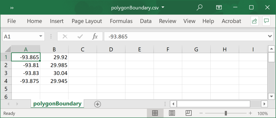
Figure 3. Subdomain Bounding Polygon CSV File.

Creating Subdomain Mesh

The main advantage of using ADCIRC subdomains is that it provides the user the flexibility to change the HEC-RAS boundary condition line and re-interpolate water level time series from the subdomain without having to go back to the full domain. In the example, below, the full domain ADCIRC mesh has about 9 million nodes while the subdomain has about 12 thousand.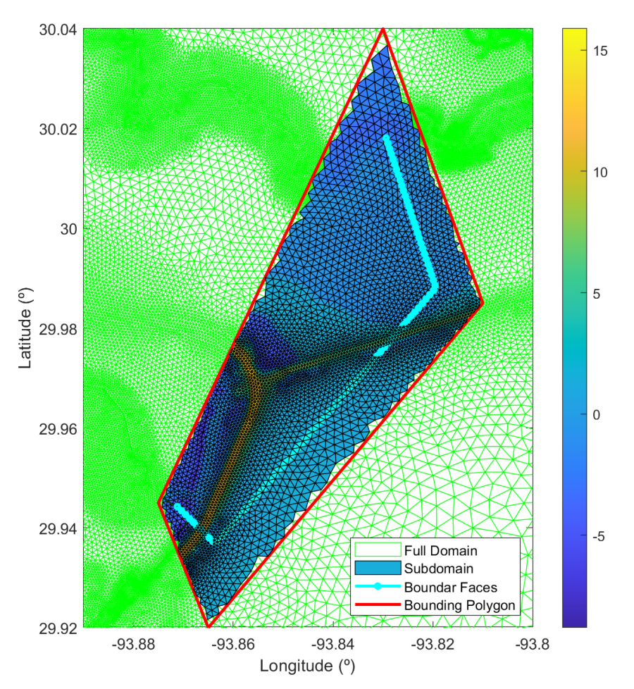

Figure 4. Example ADCIRC Full Mesh Nodes, Subdomain Nodes, Boundary Faces, and Subdomain Polygon.

The HEC-RAS nesting utility can be run from a Windows Command Prompt using the prebuilt executable, called as a library or batch script.
The example below shows how to run the Nesting.exe from the Command Prompt to create an ADCIRC Subdomain (Child Mesh) from a full Mesh (Parent Mesh) and a user-specified subdomain bounding polygon contained in a simple CSV file (Comma Separated Variables).

>Nesting.exe -gensub "Parent.grd" "polygonBoundary.csv" "Child.grd"

Similarly, the example below shows how to call the Fortran method to extract a subdomain.

parentGridFile = "Parent.grd"
polyFile = "polygonBoundary.csv"
childGridFile = "Child.grd"
call nesting_gensub(parentGridFile,polyFile,childGridFile,status,msg)

The format of the subdomain mesh file is similar to a regular ADCIRC mesh file except there is an additional column with the corresponding full mesh node indexes of each node subdomain node. An example subdomain file is shown below. The first line contains a header line. The second line contains the number of elements and nodes. The next section contains the columns, node index, node x-, y-, and z-coordinates, and corresponding full domain index number. The next section contains the 5 columns contains the element index, the number of nodes per element (always 3 in the case of ADCIRC), and the node indexes for each element. The subdomain utilized here does not contain any boundary strings since the file is not intended for model simulations.

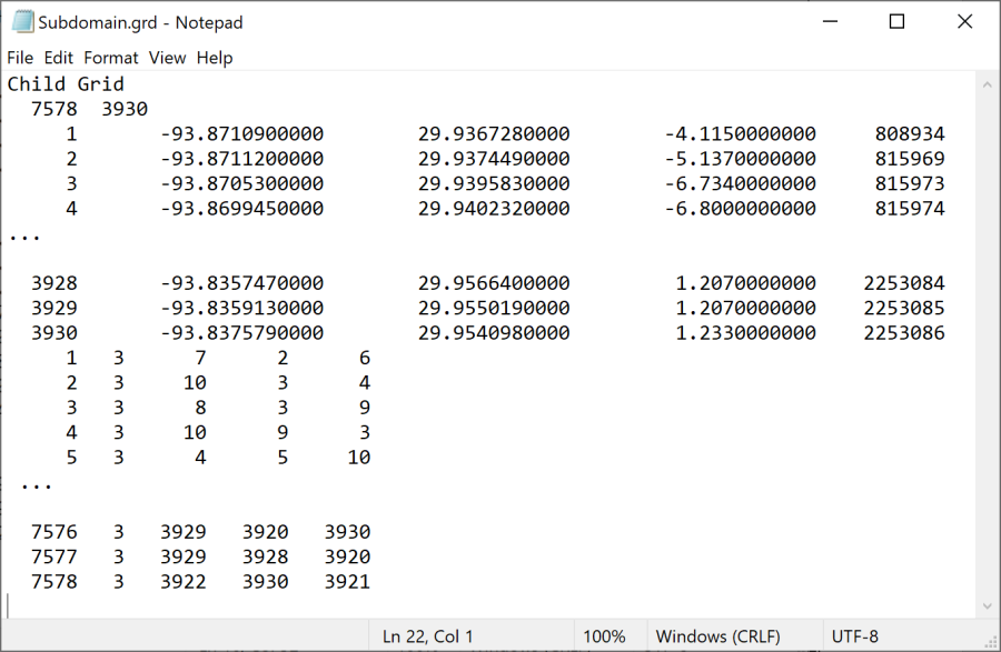
Figure 5. Example subdomain mesh file.

Extracting Water Levels on the ADCIRC Subdomain

Water levels can extracted from the full domain onto the subdomain by either running the Nesting.exe utility or calling the Fortran library. Below is an example of using the Nesting.exe utility.

>Nesting.exe -extractwse "Child.grd" "Parent_Run1.63" "Child_Run1.63"
>Nesting.exe -extractwse "Child.grd" "Parent_Run1.63" "Child_Run1.63" "Parent_Run2.63" "Child_Run2.63"

It is noted that any number of runs can be processes with a single argument

numWSEFiles = 3
childGridFile = "Child.grd"
parentWSEFiles(1) = "Parent_Run1.63"
parentWSEFiles(2) = "Parent_Run2.63"
parentWSEFiles(3) = "Parent_Run3.63"
childWSEFiles(1) = "Child_Run1.63"
childWSEFiles(2) = "Child_Run2.63"
childWSEFiles(3) = "Child_Run3.63"
call nesting_extractwse(childGridFile,numWSEFiles,& parentWSEFiles,childWSEFiles,status,msg)

Interpolating Water Level Time Series at Boundary Condition Points from Subdomain

Water levels are interpolated from the subdomain at user-specified points. Generally, the points will correspond to the face centers of a boundary. However, the points can be any points along the boundary as long as the fraction distances along the boundary are specified appropriately. An example is provided below on using the Nesting.exe utility to interpolate points from two ADCIRC runs which have been extracted onto the same subdomain.

>Nesting.exe -interpwse "Child.grd" "coordBoundary.csv" "Child_Run1.63" "wseBoundary_Run1.63" "Child_Run2.63" "wseBoundary_Run3.63" 3.280839895

If multiple runs are extracting within the same command, the runs must share the same grid. The last argument is a units conversion factor for the water levels between ADCIRC and HEC-RAS. Generally, ADCIRC water levels will have units of meters while HEC-RAS will have units of feet.

The same task can be done by calling the Fortran library.

childGridFile = "Child.grd"
pointsCoordFile = "coordBoundary.csv"
childWSEFiles(1) = "Child_Run1.63"
childWSEFiles(2) = "Child_Run2.63"
childWSEFiles(3) = "Child_Run3.63"
pointsWSEFiles(1) = "wseBoundary_Run1.csv"
pointsWSEFiles(2) = "wseBoundary_Run2.csv"
pointsWSEFiles(3) = "wseBoundary_Run3.csv"
factor = 3.280839895D0
call nesting_interpwse(childGridFile,pointsCoordFile,numWSEFiles,childWSEFiles,pointsWSEFiles,factor,status,msg)

Interpolating Water Level Time-Series from ADCIRC Save Points

Save Points are user-specified locations where various output time-series are output. Usually, the output time interval for Save Points is finer than for global output results. In some cases, it may be desirable to interpolate water levels from ADCIRC Save Points.

Triangulating Save Points

Save points are triangulated within a bounding polygon. This saves memory and time. As similar approach is adopted as in creating a subdomain in which the Save Point triangulation is stored in *.grd file with the subdomain format. Below is an example of triangulating water levels from ADCIRC Save Points using the Nesting.exe utility. 

>Nesting.exe -trisp "elev_stat.151" "polygon.csv" "SavePointTriangulation.grd"

The first argument "-trisp" is the command for Save Point Triangulation. The file "elev_stat.151" contains the coordinates of the save points. The third argument "polygon.csv" is a CSV file containing a bounding polygon for the points which will be triangulated. 

The same task can be done by calling the Fortran library as in the example below.

savePointFile= "elev_stat.151"
polyFile= "polygon.csv"
childGridFile= "SavePointTriangulation.grd"
call nesting_trisp(savePointFile,polyFile,childGridFile,status,msg)

The triangulation is computed with Delaunay triangulation. An example Save Point triangulation is shown in the figure below. It is noted that the bounding polygon for the Save Point triangulation is larger than the bounding polygon for the boundary condition faces. 

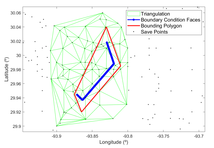
Figure 6. Example Triangulation of ADCIRC Save Points around an HEC-RAS Boundary Condition, and bounding polygon.

Extracting Water Levels on Triangulated Save Points

Water levels on the Triangulated Save Points can be extracted from the larger set of Save Points using the Nesting.exe utility with the following command:

>Nesting.exe -extractwse "SavePointTriangulation.grd" "fort.61" "TriangulationWaterLevels.61"

The second argument is the same as when extracting water levels on a subdomain from a full domain. This is possible because the Save Point triangulation is stored as a triangular unstructured mesh in the same format as the ADCIRC subdomain. 

The same task can be done by calling the Fortran library as in the example below.

numWSEFiles = 1
childGridFile= "SavePointTriangulation.grd"
parentWSEFiles(1) = "fort.61"
childWSEFiles(1) = "SavePointWaterLevels.61"
call nesting_extractwse(childGridFile,numWSEFiles,parentWSEFiles,childWSEFiles,status,msg)

Interpolating Water Levels from Triangulated Save Points

Save Points are user-specified output locations which are generally output at a higher output interval than the global output variables. 

>Nesting.exe -interpwse "Child.grd" "coordBoundary.csv" "SavePointWaterLevels.61" "wseBoundarySavePoint.61" 3.280839895

The same task can be done by calling the Fortran library.

numWSEFiles = 1
childGridFile= "SavePointTriangulation.grd"
pointsCoordFile = "coordBoundary.csv"
childWSEFiles(1) = "SavePointWaterLevels.61"
pointsWSEFiles(1) = "wseBoundarySavePoint.csv"
factor = 3.280839895D0
call nesting_interpwse(childGridFile,pointsCoordFile,numWSEFiles,childWSEFiles,pointsWSEFiles,factor,status,msg)

Specifying Spatially Variable Water Level Time Series in the HEC-RAS DSS Viewer

Spatially variable water level time series are specified using a similar approach to the stage hydrograph boundary condition from a DSS file. Spatially variable water levels can only be specified from a DSS file. Data in a different format can be imported into a DSS file using the HEC-RAS DSS viewer as discussed below. The main difference is that the spatially constant and spatially variable water level boundary condition DSS file will have multiple columns each corresponding to a different point along a boundary condition. It is important to recognize that the number of columns or water level time series does not have to match the number of faces along a boundary condition. The location of each water level time series is specified as a fractional distance from 0 to 1 along the boundary condition line. This approach allows for more flexibility in the specifying the boundary water levels. 

The first step in specifying a spatially variable water level time series is to open the HEC-RAS Unsteady Flow Data editor, select the 2D Flow Area Boundary Condition Location, and then select the Stage Hydrograph Boundary Condition Type, as shown in the figure below. 

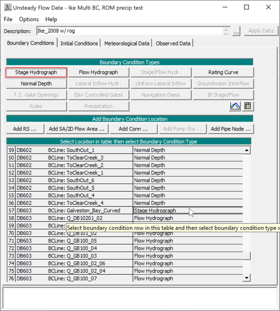
Figure 7. Selecting the Stage Hydrograph Boundary Condition in the Unsteady Flow Data Editor. 

Within the Stage Hydrograph editor, select Read from DSS before simulation, and then click on the button which reads Select DSS file and Path, as shown in the figure below. This will open the HEC-RAS DSS viewer. 

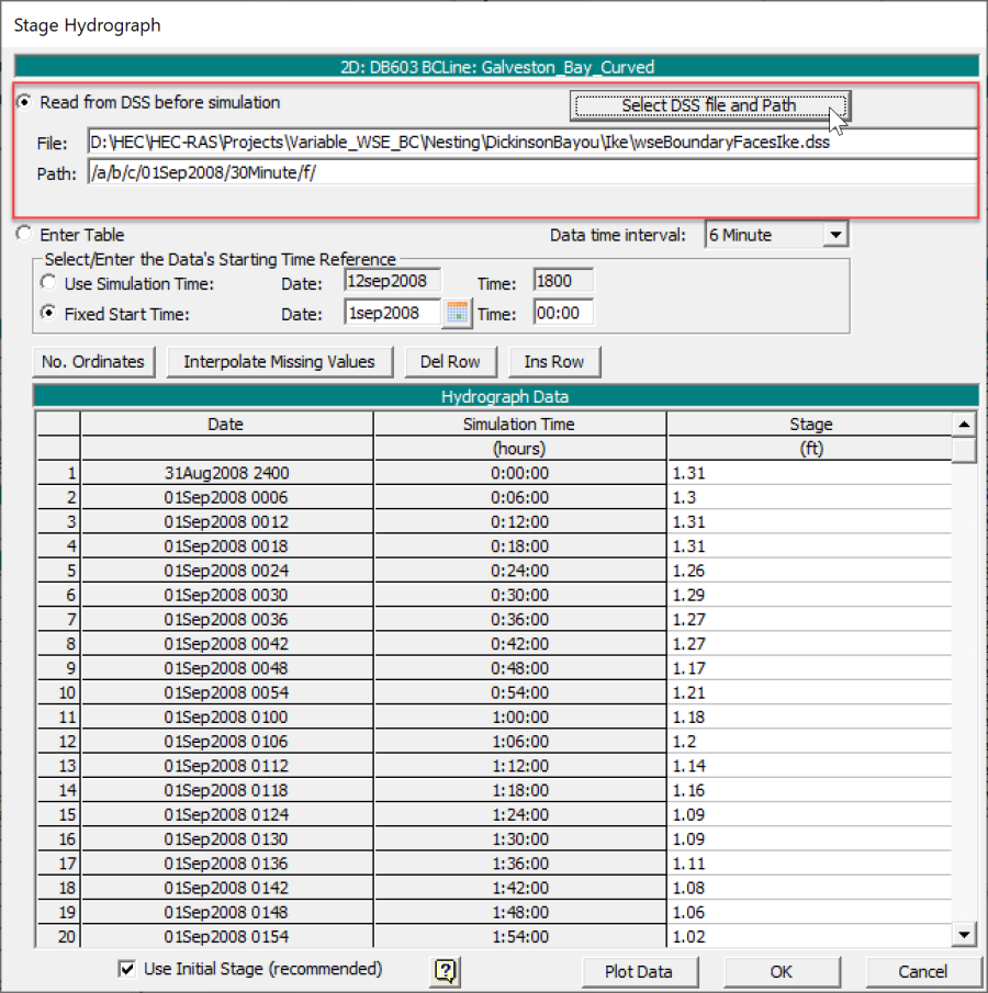
Figure 8. Selecting the DSS option for the Stage Hydrograph boundary condition.

Within the HEC-RAS DSS viewer, select the menu Utilities | Time Series Import ... as shown in the figure below. 

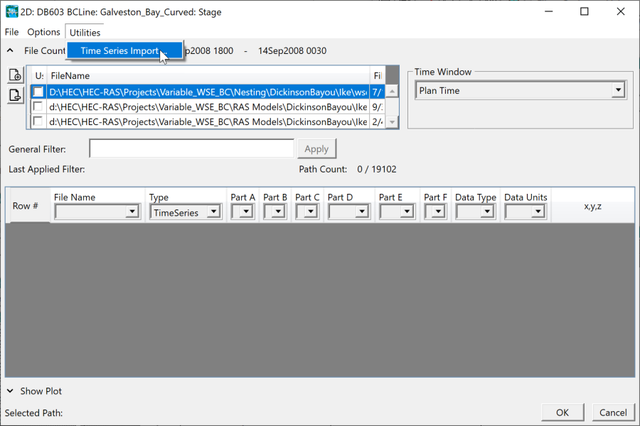
Figure 9. Selecting the option to import Time-Series in the HEC-RAS DSS Viewer. 

Within the Write Time Series Data to DSS editor, specify the path and name of the DSS file which will be used to store the water level time series (see figure below). It is recommended to use a separate file from other existing DSS file. The DSS parts A, B, C, and F are not utilized in this case but must have a value specified. For simplicity the example below uses the lower case names of the DSS path parts. The Date must be specified with the format DDMMMYYY and the time as HHMM. A constant time interval can be selected from a drop down. The units for water levels are typically feet or meters and the data type must be INST-VAL indicating instantaneous values. 

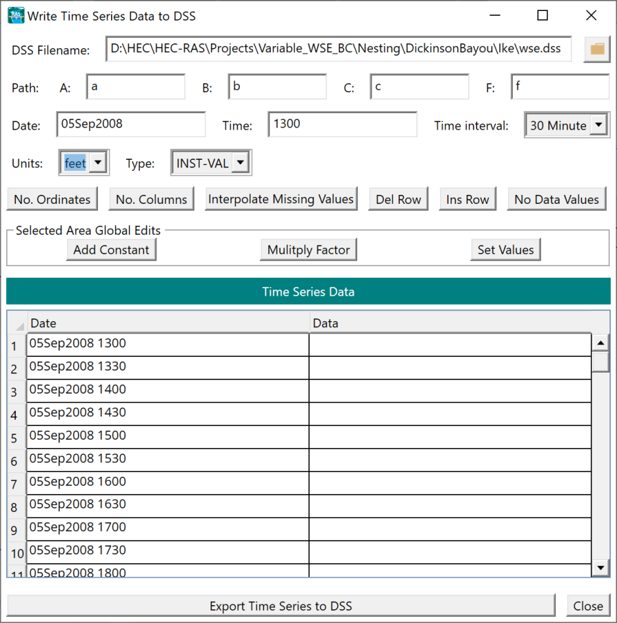
Figure 10. Example general input parameters for importing water level time series in the HEC-RAS DSS viewer. 

The next step is to select the number of columns by clicking on the button as shown in the figure below. After clicking OK, another window will appear where the time series locations specified as fractional distances along the boundary condition line are specified. These are referred to as profile numbers in DSS. The easiest way to do this is to copy-paste the values from an Excel spreadsheet. The nesting utility produces a CSV file where the first row is the fractional distances of each column. The row values cannot be copy-pasted into the HEC-RAS table, and need to be transposed first. This can easily be done in Excel.

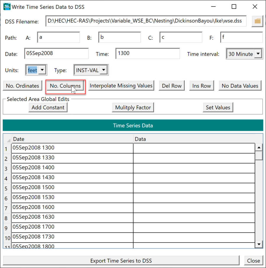
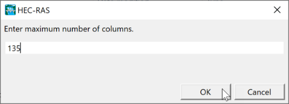
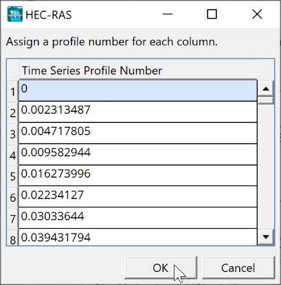
Figure 11. Entering the number of columns and face fractions as profile numbers. 

Once the number of columns and column profile numbers have been specified, the next step is to specify the time series data. This is done by selecting the top-left cell in the table and copy-pasting all of the data from a spreadsheet. Then the data can be exported into the DSS file by selecting the Export Time Series to DSS file button. Click OK in the window with the message Successfully exported time series to DSS file. Then close the Write Time Series Data to DSS editor (see figure below). 

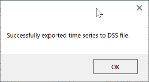
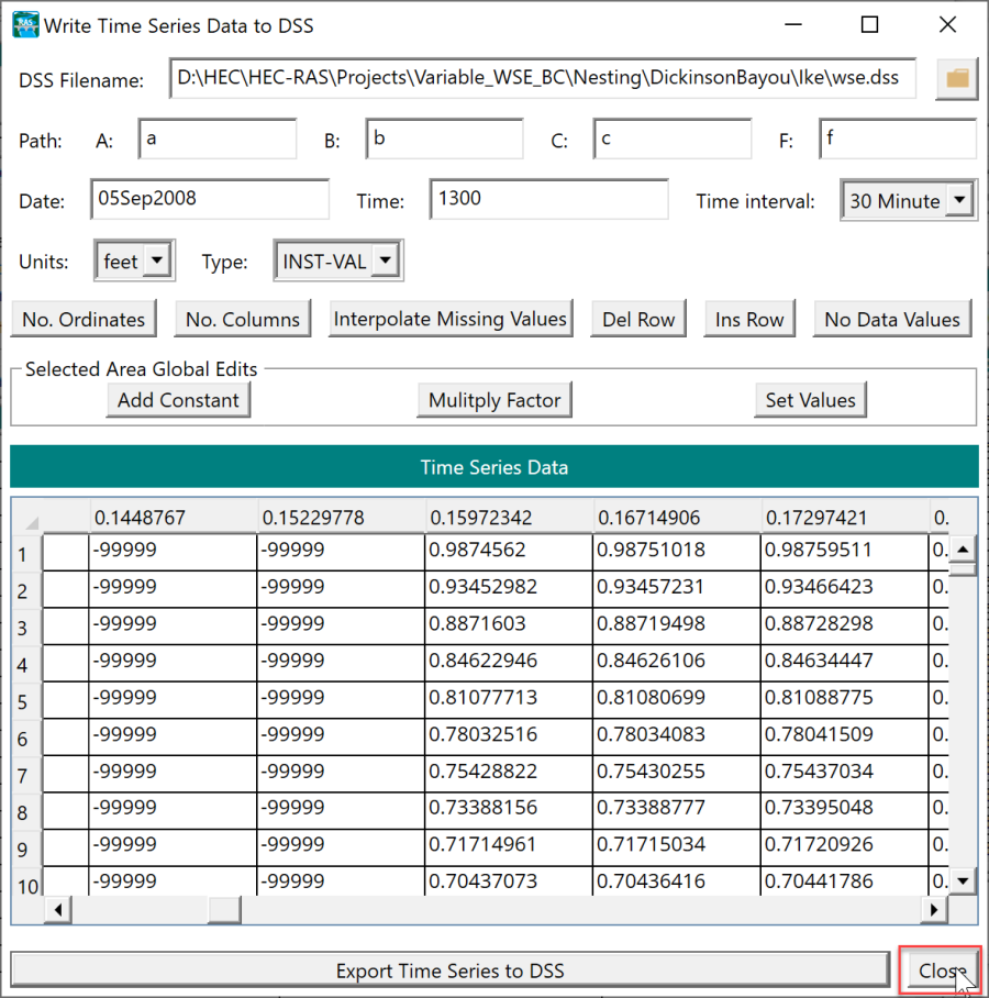
Figure 12. Copying the water level time series in the HEC-RAS DSS viewer and exporting the data to a DSS file. 

Once the water level data is exported to the DSS file, the file needs to be dataset file and path need to be selected in the HEC-RAS DSS viewer (see figure below). 

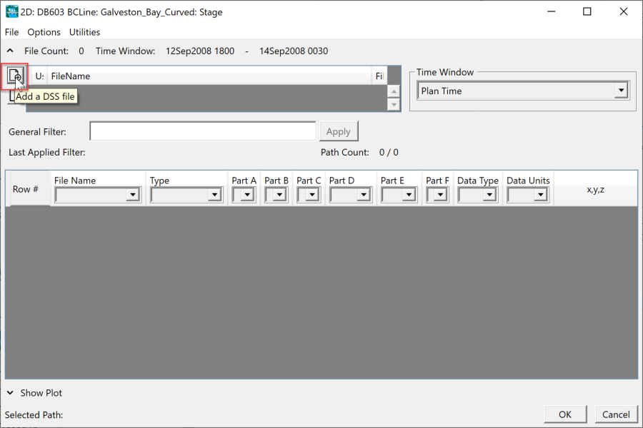
Figure 13. Selecting the DSS file with the spatially variable water level time series. 

Then the DSS record path is selected as shown in the figure below. While highlighting the appropriate DSS file, select the DSS record by double clicking on the appropriate row. If the HEC-RAS project has many DSS files, it can be easier to remove the used DSS files or unselect them to reduce the number of records to choose from. Once the DSS record is selected, click on the OK button to exit the HEC-RAS DSS viewer.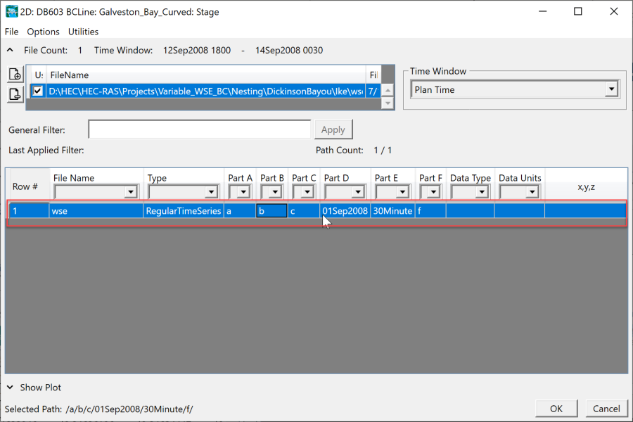 

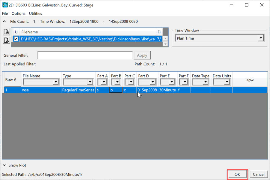
Figure 14. Selecting the DSS file and path. 

Once in the Stage Hydrograph editor, check the DSS data by clicking the Plot Data button as shown in the figure below. 

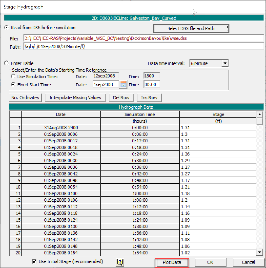
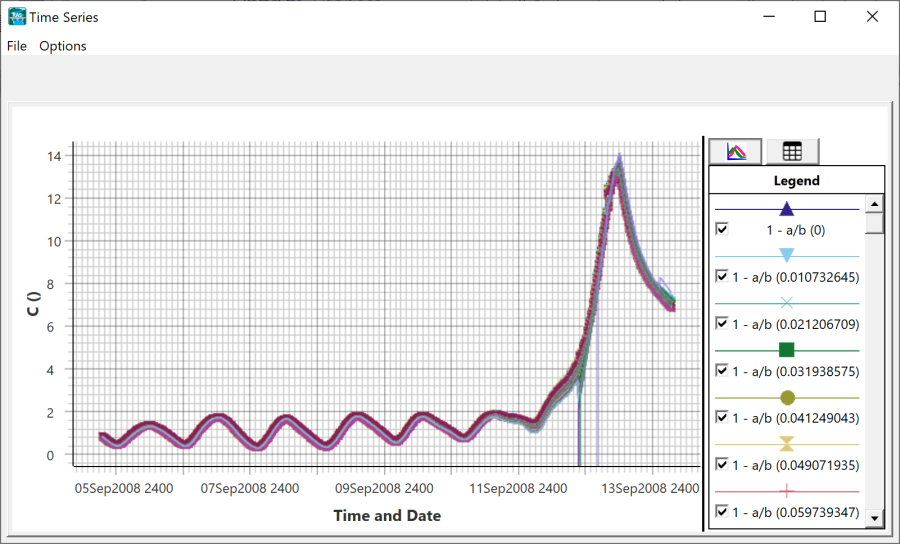
Figure 15. Plotting the DSS time series.

It is noted, that dry water surface values in ADCIRC are stored as -99999. These values will not plot well and may require the user to zoom in to viewer the data correctly. The dry values are handled inside the unsteady computational engine.