Secondary Flow

HEC-RAS 6.7 and newer have the option to simulate the momentum dispersion due to secondary flows around river bends. This section covers the HEC-RAS input related to spatial input datasets related to secondary flow. The computational options and parameters for secondary are set the 2D Flow Options tab of the Unsteady Computation Options and Tolerances window of the Unsteady Flow Data editor (see 2D Computation Options and Tolerances). When simulating secondary flow, there are two optional spatial datasets which the user can enter: (1) Land Cover Spiral Intensity Source Factor and (2) Streamline Centerline Reference Line.

Spiral Intensity Source Factor

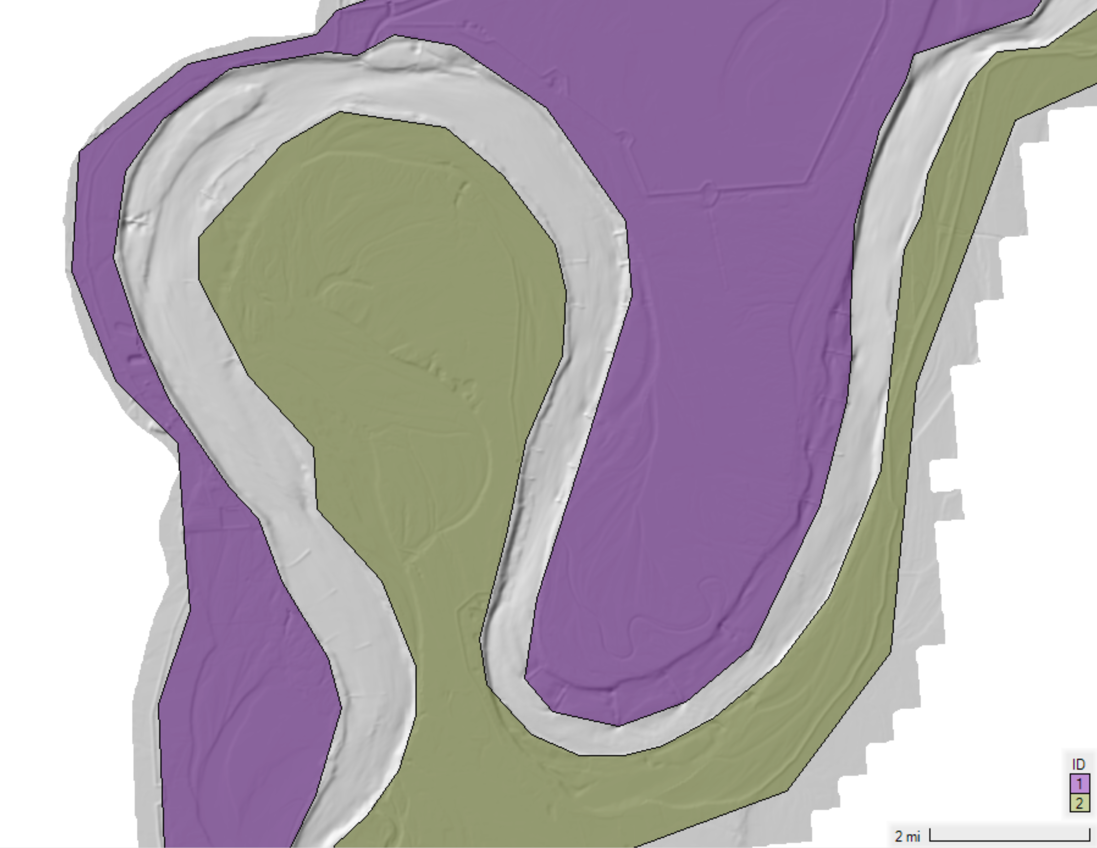
The Spiral Intensity Source Factor is useful for turning off the secondary flow effects in areas where it is not needed such as in overbank areas, small side channels, urban areas, etc. The value is multiplied by the spiral intensity source during the simulation, and should be between 0 and 1 (see image below). In addition, the parameter also speeds up the simulation because many of the calculations can be skipped for cells when the spiral intensity factor is equal to zero. The Spiral Intensity Source Factor is specified in the Land Cover layer along with ManningN and the Percent Impervious variables. The user may either choose to use the same Land Cover layer for these variables are create different layers. However, in most cases, it is most convenient to create a separate Land Cover layer for the Spiral Intensity Source Factor. To create a new Land Cover layer for specifying the Spiral Intensity Source Factor, open RAS Mapper, right-click on the Map Layers node and select Create a New RAS Layer | Land Cover Layer (as shown below).

Then import any useful classification files or simply create an empty layer as shown in the figure below. 

Then edit the layer by right-clicking the Classification Polygons node and select Edit. Draw classification polygons to specify the Spiral Intensity Source Factor. The most common use for variable is to turn off secondary flow source generation in regions where it is not needed or could cause problems. in The example below , polygons are drawn for the left and right bank regions including regions between river training structures where secondary flow is not wanted. 

Next save the changes to the classification polygons by right-clicking on the layer again and selecting Stop Editing. 

When prompted click Yes to Save Edits. 

Next enter the Land Cover Data Table by right-clicking on the Land Cover layer and selecting the menu Edit Land Cover Data Table as shown below.

In this example, the Spiral Intensity Source Factor is set to 1 in the channel (i.e. NoData), and 0 in the right and left banks of the channel (i.e. RightBank and LeftBank). 

The Spiral Intensity Source Factor can be inspected on the Land Cover dataset by hovering over the layer as shown below.  

Streamline Centerline Reference Line

By default the flow curvature is computed at each cell using the local velocity field. However, the option is provided to compute the flow curvature using a user-specified Reference Line indicating the channel streamline centerline.  The Reference Line can be created manually or extracted from a previous simulation velocity field using the RAS Mapper option Track Longitudinal Velocity at Cursor. 

To create a Velocity Track, hover over a velocity result and it will be displayed as a pink line. For secondary flow, select a region near the channel centerline and then right-click and select the menu Velocity Track (Longitudinal) | Create Reference Line. This will create a Reference Line in the corresponding geometry associated with the result. 

Next assign the name Centerline to the Reference Line (see figure below). It is important to use this exact name so that HEC-RAS can recognize it as a Reference Line for use with the flow curvature calculations. 

The figure below shows an example Reference Line called Centerline created from a Velocity Track in RAS Mapper. 

The flow curvature from a Velocity Track is typically less noisy than that from the local velocity field. However it does does not change during the simulation and therefore cannot capture changes in the flow curvature due to morphology change or simply varying flows. The figures below show a comparison of the flow curvatures estimated using the local velocity field and a river centerline (specified via a Reference Line). It's noted that the flow curvatures are zero where a user-specified Spiral Intensity Scale Factor. 

When a centerline is specified for use in calculating the flow curvature, a message will be displayed in the runtime messages "Found Centerline Reference Line for Flow Curvature" indicating the Reference Line with the name Centerline has been identified and will be used in the calculations.