Download PDF
Download page Global Boundary Conditions.
Global Boundary Conditions
HEC-RAS now has the capability to have spatially varying precipitation, evapotranspiration, and wind. Spatial precipitation, evapotranspiration, and wind data are added into the Unsteady Flow Boundary Conditions editor from the Meteorological Data Tab.
Precipitation Data
Spatial precipitation and evapotranspiration can be entered into HEC-RAS as either gridded data, point gage data, or a constant rate. The spatial precipitation and evapotranspiration data are added into HEC-RAS through the Unsteady Flow Boundary Conditions editor. From the Unsteady Flow Boundary Conditions editor, select the Meteorological Data tab and the editor will update (Figure 1). As shown in Figure 1, the user can enter precipitation data in either gridded or point gage formats.
Gridded Precipitation
To enter gridded precipitation data, first the user must select “Enable” from the “Precipitation/Evapotranspiration:” selection box, located at the upper left of the tab. Next the user must then select “Gridded” from the Mode selection box in the Meteorological Variables section of the editor. Next, click the Edit button (located to the right of the Mode selection box) (Figure 1).

Figure 1. Meteorological Data tab with Gridded DSS precipitation data.
Selecting the Edit button updates the Unsteady Flow Data editor, Meteorological Data tab to include the sections displayed in Figure 2.

Figure 2. Meteorological Data tab with Gridded DSS precipitation data and input options.
As shown in Figure 2, the user must select a data Source for the gridded data from the following options:: HEC-DSS and GDAL Raster Files (Single Raster File or Multiple Raster Files). If the “GDAL Raster Files” option is selected, that data must be in either the NetCDF or the GRIB file formats. These are National Weather Service (NWS) file formats for NWS gridded data. Once the user selects a data source, then the user should use the Open File ![]() icon next to the filename field to select the source file. If a DSS file type is selected, a DSS Pathname chooser will open once the DSS file is selected. The user must choose the DSS pathname that want to use for reading the gridded precipitation data from DSS. If the data is being read from either the NetCDF or GRIB file formats, the user must go through an import process to bring the data in before it can be used. This import process is explained in the Wind data section of this manual (both meteorological variables use is the same process for GDAL gridded data sources).
icon next to the filename field to select the source file. If a DSS file type is selected, a DSS Pathname chooser will open once the DSS file is selected. The user must choose the DSS pathname that want to use for reading the gridded precipitation data from DSS. If the data is being read from either the NetCDF or GRIB file formats, the user must go through an import process to bring the data in before it can be used. This import process is explained in the Wind data section of this manual (both meteorological variables use is the same process for GDAL gridded data sources).
Additional options for the selected source gridded data are: Ratio, Projection Override, and Units Override. The Ratio option allows the user to multiple all of the precipitation by a user specified ratio. For example, if the user enters “5” in the ratio field, then all the precipitation values will be multiplied by 5 before being used. The Projection Override option allows the user to override the horizontal projection found in the file being read. This override option is generally only needed if the software is unable to understand the projection information stored in the gridded data file. The Units Override option allows the user to override the units of the data. This option is also only needed if the software has trouble detecting the units of the data from the meta data contained within the gridded data file.
Once the gridded precipitation is defined in the Unsteady Flow Data editor (Figure 2), and saved, the user can visualize the precipitation data in HEC-RAS Mapper. Gridded precipitation can be viewed as spatial maps in both an incremental (e.g., hourly) and a accumulated form. This precipitation data is available from the RAS Mapper, Layers tree, under Event Conditions (Figure 3). Shown in Figure 3 is an example incremental precipitation map. These incremental maps can be animated over time by pressing the green Play button at the upper left of the RAS Mapper window.

Figure 3. Example gridded precipitation rates in the RAS Mapper Event Conditions.
The example provided in Figure 4-8 displays an accumulated precipitation map.

Figure 4. Example accumulated precipitation map in the RAS Mapper Event Conditions.
In addition to spatial maps, precipitation can be plotted at a point location for both incremental and accumulated precipitation data. With the two map types turned on (by checking ![]() the checkbox for the layer), from the map window right click at any location and from the shortcut menu select either: Plot Precipitation or Plot Accumulated Precipitation to open a RAS Mapper Plot of the data at the selected location. An example of a plot of incremental precipitation at a point location is shown in Figure 5.
the checkbox for the layer), from the map window right click at any location and from the shortcut menu select either: Plot Precipitation or Plot Accumulated Precipitation to open a RAS Mapper Plot of the data at the selected location. An example of a plot of incremental precipitation at a point location is shown in Figure 5.

Figure 5. Example time series of incremental precipitation rates.
An example of an accumulated precipitation plot from a point location is shown in Figure 6.

Figure 6. Example time series of Accumulated Precipitation at a point.
Once the user makes a model run, this same type of information and plotting capability is available from the Results | Event Conditions shortcut menu for a specific Plan.
Point Gage Precipitation
Users can also enter precipitation data as point gage data in HEC-RAS. This data is then interpolated in order to convert it to a gridded data form, which is how the computational engines use the data.
To enter point gage data into HEC-RAS, open up the Unsteady Flow Data editor, then select the Meteorological Data tab. The editor will update as shown in Figure 7.

Figure 7. Example Meteorological tab showing point precipitation data specified at Meteorological Stations.
To enter or edit gaged precipitation data, the user must press the Create/Edit Stations button first (Figure 7). This button will open the Meteorological Stations window, select the Table tab (Figure 8) to view the point gage Meteorological Station table. The Meteorological Stations table is used to enter the Name of the gage, and the X, Y coordinates of the gage location. Users can enter the gage location in either Latitude/Longitude, or in the project X, Y coordinate system (this is based on the horizontal coordinate system setup for the RAS Mapper project). Users must first fill out all of the gage Point Names (or gage locations). The tab labelled “Detailed,” allows the user to create one gage at a time, rename a gage, and delete a gage.

Figure 8. Meteorological Stations editor showing the Geographic and Projected station coordinates.
Then, under the Meteorological Variables section of the editor, the user should select the Point method from the Precipitation Mode dropdown. Next press the Expand/Edit button to view the additional point data information. The Point Time Series Data will open, allowing the user to select one of the Interpolation Methods and for each individual point gage in the Point Time Series Data table (Figure 9), click the Edit ![]() button to edit or enter data for each of the individual point gages. See Figure 4-13 below.
button to edit or enter data for each of the individual point gages. See Figure 4-13 below.
Figure 9. Example precipitation data specified at Meteorological Stations.
For each of the gages that the user would like to use for the event being modelled, the user must Edit each of the individual point gages in order to define the precipitation and turn that gage on for use. Click the Edit ![]() button to open the Point Meteorological Time Series window for the selected gage (Figure 10).
button to open the Point Meteorological Time Series window for the selected gage (Figure 10).

Figure 10. Example DSS time series of hourly precipitation data.
As shown in Figure 10, the user must also select the Source for the data. The data Source can be: DSS (HEC-DSS), Table, or a Constant value (e.g., 1.5 in/hr). If DSS is selected, then the user must select the appropriate HEC-DSS file and also the specific HEC-DSS pathname that contains the correct data for the specific gage and the event being modelled.
For the point gage data to be used in the analysis, the user MUST check the Use this Met Station Point location ![]() checkbox. If this box is not checked, then the selected gage (e.g., ALVIN BUSH DAM in Figure 4-14) will not be used in the analysis. This option allows user to turn on or off various gages in order to experiment with the effect of different gages being included or not. The user must check this checkbox for all the desired gages to be used in the analysis. From the Point Meteorological Time Series window, click OK to return to the Unsteady Flow Data editor, Meteorological Data tab, and continue editing or entering data for each of the individual point gages (Figure 10).
checkbox. If this box is not checked, then the selected gage (e.g., ALVIN BUSH DAM in Figure 4-14) will not be used in the analysis. This option allows user to turn on or off various gages in order to experiment with the effect of different gages being included or not. The user must check this checkbox for all the desired gages to be used in the analysis. From the Point Meteorological Time Series window, click OK to return to the Unsteady Flow Data editor, Meteorological Data tab, and continue editing or entering data for each of the individual point gages (Figure 10).
Once all of the desired point gages data has been entered, and the checkboxes have been checked to use those gages, the last steps are to set the Rasterization Parameters and to select the Interpolation Method. To set the rasterization parameters, press the button labeled Rasterization Parameters (Optional) from the Meteorological Data tab. The Raster Parameters editor opens (Figure 11).

Figure 11. Raster Parameters editor.
As shown in Figure 4-15, the user can define the coordinate extents for how the point gage data will be rasterized. There are several options for defining the raster coordinate extents. The first option is to completely define the extents and the cell size to use. This first option is accomplished by entering a Left and Top coordinate (in the coordinate system established for the model in RAS Mapper), entering the number of Rows, Cols (columns), and the Cell Size. Note, the Cell Size is entered in feet when working in English units, and in meters when working in metric units. The second approach is to use one of the three buttons on the right-hand side of the window. These three options are: Fix Raster Parameters based on the current Met Station Extent, Fix Raster Parameters based on the current Met Stations and Current Geometry Extent, and Clear (use Met Stations Extent at runtime). The last option is often used for real time forecasting, in which the number of available gages that are recording may change.
To understand exactly what is produced by the rasterization of the point gage data, press the button labeled Plot Raster Extents. The Meteorological Stations window opens (Figure 12), which provides a plot for visualizing what the extents would be for each of the possible options. See an example below in Figure 12. Click OK to save the selected rasterization of point gage data and return to the Unsteady Flow Data editor, Meteorological Data tab (Figure 11).

Figure 12. Example Meteorological stations plot.
In order to complete the point gage precipitation method, from the Unsteady Flow Data editor, Meteorological Data tab, the user must select the Interpolation Method (Figure 9). The four point gage Interpolation Methods available to the user are: Thiessen Polygon, Inverse Distance Squared, Inverse Distance Squared (Restricted), and Peak Preservation.
The Thiessen Polygon method is the traditional method often used in hydrologic modeling. This method draws a line between two point gages and finds half the distance between each gage. This distance calculation is done for all of the gages and then polygons are formed by the linear bisection lines between the gages. HEC-RAS only does this in order to figure out which gage should be used for the pattern of the rainfall event. If a 2D cell is closet to a specific gage (inside that gages’ polygon), then that gage will be used for the pattern (intensity versus time) for the rainfall event. However, for the storm total rainfall at each cell, the Inverse Square of the Distance method is used in order to get a weighted storm total rainfall for each cell. That storm total is then applied to the nearest gages’ pattern in order to define the rainfall for that specific cell.
The Inverse Square of the Distance method computes a weighted depth of rainfall for each time period individually by using the inverse square of the distance weighting method for all of the gages near a specific cell. If the rainfall data is hourly, then the inverse square of the distance weighting method is done individually for each one hour time step.
The Inverse Distance Squared (Restricted) method does the same thing as the Inverse Square of the Distance method, except it first triangulates all of the gages. Then, if a cell lies inside of a specific triangle, then only the three gages that form the triangle are used in the storm weighting process. This method prevents gages that are far away from being used and limits the interpolation to the three closest gages to the cell.
The Peak Preservation method is an attempt to retain the intensities within a storm as it moves across a watershed. The Inverse Square of the Distance and Inverse Distance Squared (Restricted) methods have the problem of diminishing the rainfall intensities when the timing of the rainfall is different at each of the gages being used for the interpolation. The Peak Preservation method takes all the gages being used for a particular cell and finds the center of mass of the precipitation for each of the gages. Next all the gaged data is lined up by the center of mass. Then the data is interpolated on a time step by time step basis. Finally, the interpolated data is shifted back to the correct time to account for the location of the cell between the gages.
In order to test the different interpolation methods, the HEC-RAS team has added the ability to visualize the interpolation of the precipitation data inside of RAS Mapper. RAS Mapper (in HEC-RAS Version 6.0) now contains a layer in the Layers window, called Event Conditions. This new layer will allow the user to view and/or animate precipitation data (gridded and point data) and wind data. To view the Point Precipitation data and its resulting interpolated values, save the precipitation data (by selecting the File | Save Unsteady Flow Data menu option), open RAS Mapper, and from the Layers window, turn on the precipitation layer that corresponds to the data entered into the Unsteady Flow Data editor. An example of this for Point Precipitation, using the Thiessen Polygon interpolation method is shown in Figure 13.

Figure 13. Example map of precipitation rates interpolated with the Thiessen Polygon method.
HEC-RAS Mapper has a layer for the incremental precipitation, called Precipitation. There is also a layer for the cumulative precipitation, called Precipitation (Accumulated). User can turn on ether of the precipitation layers. These layers can be animated or a specific point in time can be selected. Additionally, the user can right click on the map and request one of three different time series plots. The time series plotting options are: Plot Precipitation (this is the incremental precipitation versus time plot), Plot Accumulated Precipitation (accumulated precipitation versus time), and Compare Precipitation Methods (accum) (this option plots all four of the point precipitation methods for the accumulated rainfall versus time). Shown in Figure 14 is an example of an Incremental Precipitation time series plot.

Figure 14. Example time-series plot of incremental precipitation rates.
Shown in Figure 15 is an example Accumulated Precipitation versus Time plot.

Figure 15. Example time-series plot of Accumulated Precipitation.
Shown in Figure 16 is an example of Accumulated Precipitation versus Time for all four available precipitation interpolation methods.
Figure 16. Compared of Accumulated Precipitation time-series for different interpolation methods.
Additionally, users can right click on the Precipitation layer and select the menu option called: Rasterization Parameters. This menu option will bring up a submenu allowing the user to select one of the four point precipitation interpolation methods, define how the program extrapolates outside of the point gage data, select a resampling technique, and also select the cell size to use when rasterizing the precipitation data (default is a cell size of 2 kilometers). Users can select a smaller cell size for rasterizing the precipitation data; however, there must be enough point gages close enough together in order to justify using a smaller precipitation cell size.
Evapotranspiration Data
Evapotranspiration data represents the potential evapotranspiration (PET) and is applied first to the surface water (storage areas, 1D XS's, and 2D cells) and then the soil moisture in the Deficit and Constant or Green and Ampt infiltration methods. The PET is not utilized in the SCS Curve Number method. Additionally, PET is an option, not a requirement, for these two methods. Evapotranspiration data can be entered as gridded data, point gage data, or just a constant rate. The methods of entering the evapotranspiration data into the Unsteady Flow Data editor is similar to precipitation, as described above.
Wind Forces
Wind forces can be incorporated in both 1D and 2D unsteady flow modeling. Wind data (speed and direction) can be entered as either gridded data or point gage data, just like precipitation data described above. If the user enters wind data into the Unsteady Flow Data editor, that data will be used and wind forcing will be applied to all 1D river reaches and 2D flow areas that are using any of the 2D flow solvers. However, it is recommended to use the Shallow Water Equation solvers in combination with wind forcing.
Gridded Wind Data
To enter gridded wind data (speed and direction), open the Unsteady Flow Data editor and select the Meteorological Data tab (Figure 4-21). From the Wind Forces dropdown select from one of the three options: No Wind Forces, Speed/Direction, and Velocity X/Y. If No Wind Forces (Default) is selected, then no wind forces are applied to the data set. If Speed/Direction is selected, then the user must enter the wind data as separate speed data and separate direction data, based on degrees from north (North is zero degrees, East is 90 degrees, etc.). If the user selects Velocity X, Y, then the wind data is entered as a velocity X component and a velocity Y component for each grid. The Velocity X, Y approach will define the magnitude and direction. An example with wind defined by Speed/Direction is shown below in Figure 17.

Figure 17. Example Meteorological tab with wind defined as Speed and Direction.
As shown in Figure 17, the user must first define the Mode for entering the data, such as: Point, Gridded, or Constant. In the example shown in Figure 17, the wind data is being entered as Gridded data. Gridded data requires a separate grid for the Wind Speed and the Wind Direction. The options for the Source of the wind data are: DSS, Single Raster File, and Multiple Raster Files.
If DSS is selected the user must specify the HEC-DSS file containing the data, and the DSS pathname pointing to the gridded information. If a Single Raster File is selected, that means a single Raster file contains all of the spatial data for the entire time window of the event being modelled. The Raster files can be either a NetCDF file or a GRIB file (National Weather Service formats). If the Multiple Raster Files Source is selected, that means that more than one file contains the data for the entire time window being modelled. NetCDF and GRIB file formats are also available for this data source.
For the Raster file data source, the user must specify the location and name of the file(s), as well as which group within the file contains the specific data (speed or direction, velocity X and velocity Y). As shown in Figure 17, once the user has specified “Gridded” data and the source as “GDAL Raster Files,” then the user must press the Import Raster Data button to go through the import process. When the Import Raster Data button is pressed, then an Import Gridded Data window will open, as shown in Figure 18.

Figure 18. Import Gridded Data editor.
As shown in Figure 18, the user selects from importing either a Single Raster File that contains all the data or Multiple Raster Files. Once either the Single or Multiple Raster files are selected, the user presses the Import Grids button to import the data. If the data is from a NetCDF file, a new window will appear, asking the user to select which individual data set should be imported from the discovered data sets in the file. For example, if the user is trying to import the Wind Speed data, then the header or data set that contains the wind speed data (usually labeled “US” should be selected. If the user is trying to import the wind direction data, then the header or data set that contains the wind direction data (usually labeled “UD” should be selected.
Because the NetCDF and GRIB file formats can contain meta data in different formats, from the Unsteady Flow Data editor, Meteorological Data tab (Figure 4-21) there are two options to override certain pieces of needed information. These options are: Projection Override and Units Override. These fields are optional and should only be used to override the projection and/or units of the data.
Once the gridded data is entered into the Unsteady Flow Data editor and saved, the user can open HEC-RAS Mapper and visualize the gridded wind data from the Event Conditions layer. This data can be animated in time. Users can also right click on the map and ask for a time series of the wind speed and direction at that location (this will bring up two separate plots, one for speed and one for direction). An example plot of a gridded wind field is shown in Figure 19 below.

Figure 19. Example map in RAS Mapper of gridded winds.
Gridded wind data can be created from ADCIRC wind files using the HEC-RAS nesting utility (https://github.com/HydrologicEngineeringCenter/ras-nesting-util). The utility is available as binaries or can be compiled and run directly from the source code. The nesting utility allows the user to extract winds from an ADCIRC model for a smaller subdomain of the whole mesh. The subdomain wind data can then be interpolated using external utilities and converted to the GDAL NetCDF format to import into HEC-RAS.
Point Gage Wind Data
Users can also enter wind data as point gage data in HEC-RAS. This data is then interpolated in order to convert it to a gridded data form, which is how the computational engines use it. Point gage data for wind is entered in the same manner as point gage precipitation data, which is documented above. Please refer to the Point Gage Precipitation Data section of this manual to understand how to enter point gage data for wind gages.
Atmospheric Pressure Data
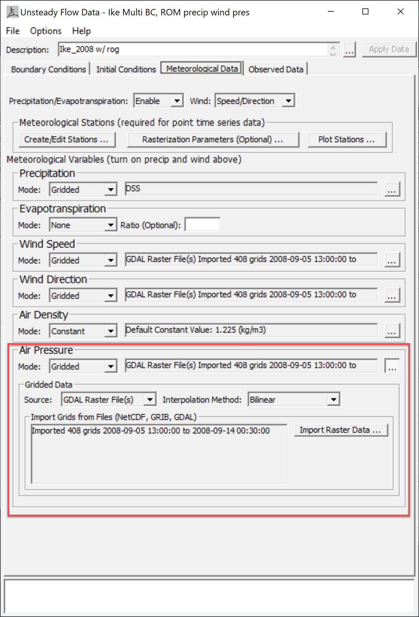
Gradients in atmospheric pressure act as a driving force for 2D flow models. Atmospheric pressure forcing is important when simulating coastal storms, hurricanes/cyclones when the gradients of atmospheric pressure can be significant. It is not recommended to use HEC-RAS as a coastal model since it does not have wave forcing and other processes. HEC-RAS should only be used for in areas where waves are not significant. Atmospheric pressure data can be entered in the Meteorological Data tab of the Unsteady Flow Data editor (see figure below). Atmospheric forcing can be applied to any of the hydraulic flow models. However, it is recommended that the shallow water models be used in combination with atmospheric pressure. The methods for specifying atmospheric pressure data in HEC-RAS are very similar to the other meteorological data described in the sections above. The data entry modes for Atmospheric pressure are Constant, Point, and Gridded. If default mode is constant in which the user may enter a single constant value. It is noted that in this mode the atmospheric pressure does not provide any forcing. The Constant mode option is provided for completeness and to support future features in HEC-RAS. The Point and Gridded modes work essentially the same for atmospheric pressure as they do for the other meteorological variables.
As with the other Meteorological Variables, Atmospheric Pressure is first interpolated onto a meteorological grid, and then interpolated on to cell centers. The gradients of atmospheric pressure are then computed at each face using the cell values.
Similar to wind data, gridded atmospheric pressure data can be created from ADCIRC files using the HEC-RAS nesting utility (https://github.com/HydrologicEngineeringCenter/ras-nesting-util). The utility can be used to extract atmospheric pressure from the whole ADCIRC domain to a smaller subdomain covering the HEC-RAS geometry. The subdomain atmospheric pressure data can then be interpolated using external utilities and converted to the GDAL NetCDF format to import into HEC-RAS.