Download PDF
Download page Initial Conditions.
Initial Conditions
Initial conditions for 2D flow areas can be accomplished in several ways. Two-dimensional (2D) flow areas can: start completely dry; be set to a single water surface elevation; set by using a Restart File from a previous run; set by interpolating results from an existing HEC-RAS Results File for a specific Plan, date, and time; 2D flow areas can be established using the 2D Initial Conditions Ramp up Time option at the beginning of the run; or by using Initial Conditions Points with a specified water surface.
Dry Initial Condition
Nothing needs to be done to start a 2D flow area in a dry condition as this is the default option. The name of the 2D flow area will show up under the Initial Conditions tab of the Unsteady Flow Data editor (see figure below). If the initial condition elevation column is left blank, this tells the software to start the 2D flow area dry. Note: A 2D area connected directly to the upstream end or the downstream end of 1D reach cannot start dry (see previous discussion).
Single Water Surface Elevation
When the single water surface elevation option is used, every cell that has a lower terrain elevation than the user established water surface will be wet (with a water surface at that elevation), and cells with a terrain elevation that is higher than that water surface will be dry. To use this option, enter the water surface elevation desired in the Initial Elevation column of the Unsteady Flow Data editor, Initial Conditions tab and in the row for the 2D flow area (see figure below).
Restart File
A Restart File can be used to establish initial conditions for an entire simulation. Refer to the Unsteady Flow Data Editor section of the HEC-RAS User’s Manual for more information regarding the Restart File option. If a previous run has been made, and the option to write out a Restart File was used, then a Restart File can be used as the initial conditions for a subsequent run. The Restart File option has been modified in HEC-RAS Version 6.0 to allow for restarting 2D flow areas in addition to all of the 1D flow elements in HEC-RAS. For 2D modeling, the Restart File will contain a water surface elevation for every cell in the model. Additionally, restart files can be generated using either of the 2D equation sets (Full Saint Venant or Diffusion Wave), and can be used to start a model with a different equation set (i.e., the user can run the original run with the Diffusion Wave option and create a Restart File, then start up a model that uses the Full Saint Venant equations from that restart file). See the section on Initial Conditions in Chapter 8 of the HEC-RAS Version 6.0 User’s Manual for more information on how to use the Restart File option.

Interpolation from Previously Computed Results
Another way to establish the initial conditions of a model (1D, 2D, or combined 1D/2D), is to use the interpolated results from a previously run Plan. This option is extremely flexible in that it does not have to be from the Plan being run and the model geometry being used for the plan can be edited and the compute will still work without modification. The user selects a previously computed Plan, Date, and time of an existing results file. At run time, HEC-RAS will interpolate water surface elevations, velocities, and flows, as needed from the HEC-RAS Mapper output data for the Plan. For example, 2D cells get an interpolated water surface elevation at the cell computation point if the cell is wet. 2D faces get an interpolated normal velocity at the center of the face for each face that is wet. 1D cross sections get an interpolated water surface at the location where the river line crosses the cross section. 1D cross sections get an interpolated flow for that cross section. And 1D Storage Areas get and average water surface computed from all the water surfaces contained within the storage area polygon.
To use the option to “Interpolate from Previously Computed Results File,” go to the Initial Conditions tab on the Unsteady Flow Data editor (see figure below).

As shown in the figure above, to use this method for initial conditions select the Results Filename option. Once this option is selected the user must first pick the HDF output file from the previously run Plan that they want to interpolate an initial condition from. The HDF output files will follow this convention: “projectname.p##.hdf”. This is the output file that HEC-RAS Mapper uses to create all of the results maps. The next step is to pick an available Results Profile (Date and Time) from the selected output file.
As stated previously, at run time HEC-RAS will interpolate results from the computed results of the selected plan/date/time and set those results for the currently run Plan. This method will work even if the 2D mesh, 1D cross sections, or storage areas are modified. This makes the Interpolation from Previously Computed Results option the most flexible way to establish an initial condition when the model contains 2D flow areas.
2D Flow Area Initial Conditions Ramp Up Option
The unsteady flow capability in HEC-RAS has always had an option to run a model warm-up period. The model starts with the initial conditions and holds all of the boundary conditions constant, based on their value at the beginning of the simulation, and then runs a series of time steps with the constant inflow. This warm-up period allows the model to establish water surface elevations and flows that are consistent with the unsteady flow equations being applied. If there are any lateral structures that have flow (based on the initial conditions) going across the structure, this flow will transition from a very small flow to the full computed flow over the duration of the warm-up period. This unsteady flow capability can reduce shocks to the system, especially in 1D river reaches.
Two-dimensional (2D) flow areas have an additional option called Initial Condition Ramp Up Time. If a 2D area has external boundary conditions (flow hydrographs or stage hydrographs) or links to 1D elements, in which flow will be going into or out of the 2D area right from the start of the simulation; then, the 2D flow area Initial Condition Ramp Up Time must be turned on to get flow through the 2D area in order to establish its initial conditions before the start of the simulation (or even before the start of the overall model warm-up time). The 2D flow area Initial Condition Ramp Up Time is a separate option for the 2D flow areas (separate from the overall model warm-up option). To use this option, select the Options menu from the Unsteady Flow Analysis window, then select Calculation Options and Tolerances. The HEC-RAS Unsteady Computation Options and Tolerances (Figure 4-26) window opens. Select the 2D Flow Options tab (Figure 4-26). The user enters a total ramp up time in the Initial Conditions Ramp Up Time (in hours) field. Additionally, the user must enter what fraction of that time is used for ramping the 2D boundary conditions up from zero to their first value (i.e., a stage or a flow entering the 2D Area). This is accomplished by entering the fraction in the Boundary Condition Ramp Up Fraction (0 to 1) field. The default value for the ramp up fraction is 0.1 (10 % of the ramp up time).

Say, for instance, that a 2D area has an upstream flow boundary and a downstream stage boundary and the user has entered a two hour Initial Conditions Ramp Up Time with the Boundary Fraction at 0.5 (50%). Assume for this example that the first flow on the flow boundary is 1,000cfs and the first stage of the downstream boundary has an elevation that corresponds to 10ft of depth above the invert of the stage boundary (the invert is the lowest point along any part of the faces that make up the boundary). For the first hour of the initial conditions, the flow will increase linearly from 0cfs up to 1,000cfs. Then for this example, the downstream stage boundary will transition from a depth of 0ft up to a depth of 10ft (and even though this is a “downstream” boundary, if the 2D area started out dry, then flow will initially come into the 2D area). For the second hour, the flow will held at 1,000cfs upstream and the depth at 10ft downstream.
The initial conditions, if any, are computed separately for each 2D area (in a “standalone” mode). The flow and stages from any boundary conditions directly connected to the 2D area are taken into account. The flow and/or stage from any 1D river reach (that is directly connected) is taken into account to the extent possible. However, flow from any lateral structure or storage area connections is not taken into account during this part of the computations. Flow crossing a hydraulic structure that is internal to the 2D area is computed. If the user has entered a starting water surface for the given 2D area, that water surface is used before applying the 2D initial conditions ramp up time. Otherwise the 2D area starts out dry.
In addition to establishing the initial conditions within 1D river reaches and 2D flow areas, it is a good idea to turn on the overall model warm up option. By enabling this option, the program will hold all inflows constant, then solve the entire unsteady flow model together (1D and 2D) to get the unsteady flow equations and hydraulic connections to settle to a stable initial condition before proceeding with the event simulation. The overall model warm up is turned on under the General (1D Options) tab from the Unsteady Flow Analysis window, Options menu, Calculation Options and Tolerances. The user turns this option on by entering a value into the field labeled Number of warm up time steps (0 – 100,000). This entered value is for the number of time steps the user wants the model to run for the warm up period. From the General (1D Options) tab, there is also an option to put in a computation interval to use during the model warm up period (Time step during warm up period (hrs)). If this field is not set, then the program uses the default computation interval set by the user from the Unsteady Flow Analysis window. However, sometimes it can be very useful to use a smaller time step during the model warm up period in order to get the initial conditions established without going unstable.
Initial Conditions Points
Initial Conditions Points (IC Points) are used in HEC-RAS to establish an initial water surface. To use the IC Points option, you create IC Points in RAS Mapper and then provide the water surface elevation for each point in the Unsteady Flow Editor.
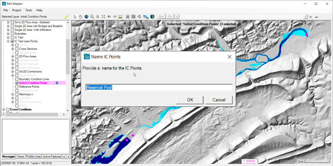
The Initial Conditions Points layer for each geometry is available for editing using the tools in RAS Mapper (or the Geometric Data Editor). To create a IC Points in RAS Mapper, Start Editing the Initial Conditions Points layer and then use the Add New Feature tool to add a point. Once a point is created, you will be asked to provide a Name, as shown below.
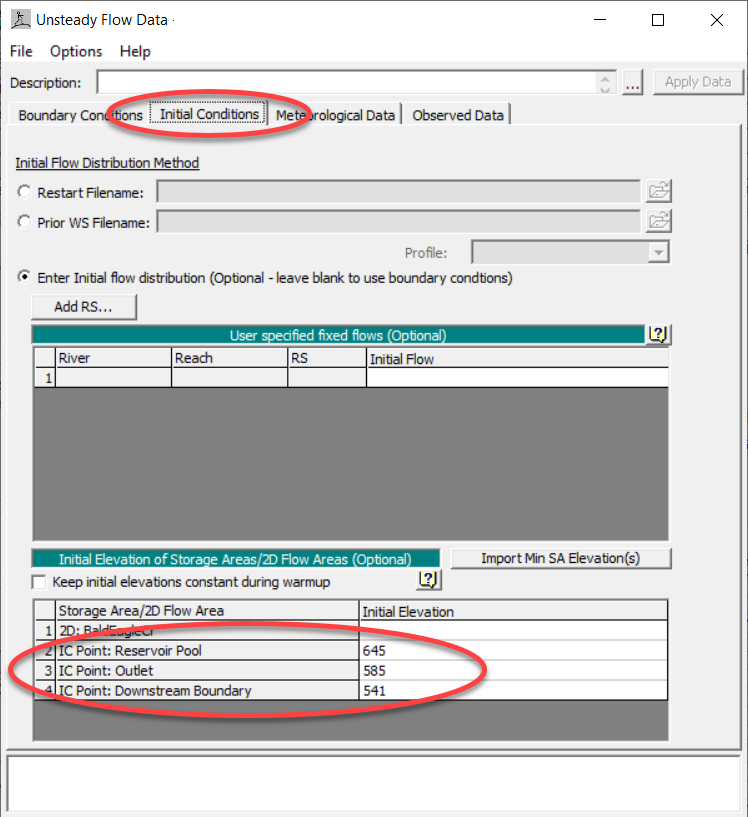
After creating IC Points, open the Unsteady Flow Data Editor, shown below. Navigate to the Initial Conditions tab, and enter an Initial (water surface) Elevation for each point.
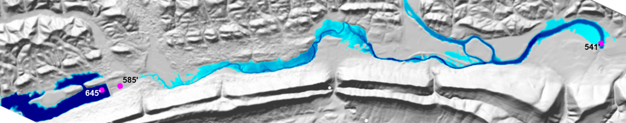
Plotting the Initial Elevations in RAS Mapper is shown in the figure below.
Prior to running the simulation, the specified Initial Elevations will be used to compute the initial conditions water surface. How the initial water surface is computed, depends on the layout of the IC Points - whether the points are considered Upstream Points or the most Downstream Point. There is only 1 Downstream Point and it is selected by having the lowest elevation based on the underlying terrain.
- Upstream Points - there are no IC Points hydraulically upstream from Upstream Points. The water surface elevation at these points are projected horizontally upstream until they intersect with high ground or reach the booundary.
- These points will fill a pool with a horizontal water surface and are appropriate upstream of hydraulic structures like dams.
- The water surface is computed assuming normal depth is achieved, using a constant flow per unit width (q) approach to Manning's equation to connect with the most Downstream Point. This flow per unit width computation procedure is described in more detail below.
- If the computed water surface profile would create a backwater on another tributary, the higher water surface is projected horizontally until it intersects the tributary water surface.
- Downstream Point - there are no IC Points hydraulically downstream from the Downstream Point. The water surface elevation at this point is projected horizontally downstream to the boundary or until it intersects with high ground. Therefore, you should always specify a IC Point at the downstream boundary.
Once the initial water surface is computed for the main river network, it is used to seed a wave fill algorithm to propagate the computed water surface out into the floodplain. The wave fill is similar to a flood fill in that the seeded water surface elevation attempt only fill connected areas, however, the wave continues to interpolate water surface elevations based on neighboring cell values to allow for a sloped water surface.
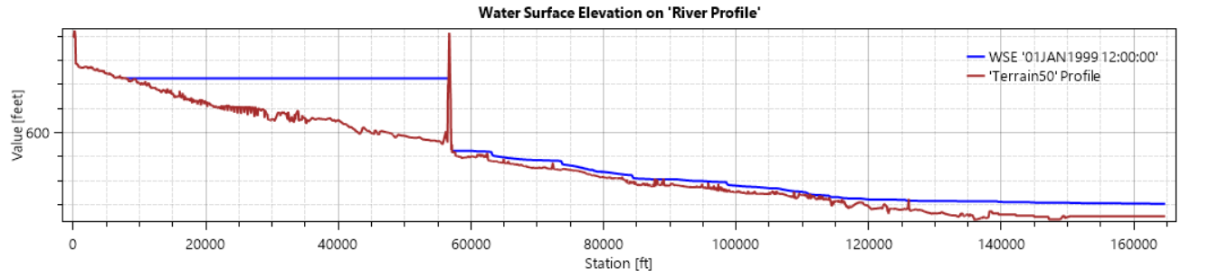
The initial conditions water surface will be computed and used at the starting water surface for the unsteady flow simulation. An example initial conditions water surface is shown below.
Note that if the initial conditions water surface is jagged or does not look appropriate, you can set the Number of Warm Up Time Steps >0 to run the the model holding all flows constant but using the initial water surface to set the elevations throughout the model.
Flow Per Unit Width Computation Procedure
The Flow per Unit Width Computation Procedure used in RAS Mapper to establish initial conditions has several assumptions built into the method. First, is that that normal depth is achievable given the prescribed geometry such that Manning's equation (show below) is appropriate.
| Q=\frac{1}{n}AR^{2/3}S_f^{1/2} |
Writing Manning's equation out with more terms (d, depth and w, width), we have the following equation.
| Q=\frac{1}{n}dw*[\frac{dw}{w+2d}]^{2/3}S_f^{1/2} |
Further, using the wide-channel assumption (w >> d), we can rewrite Manning's equation as a flow per unit width (q), as shown below.
| q=\frac{1}{n}d^{5/3}S_f^{1/2} |
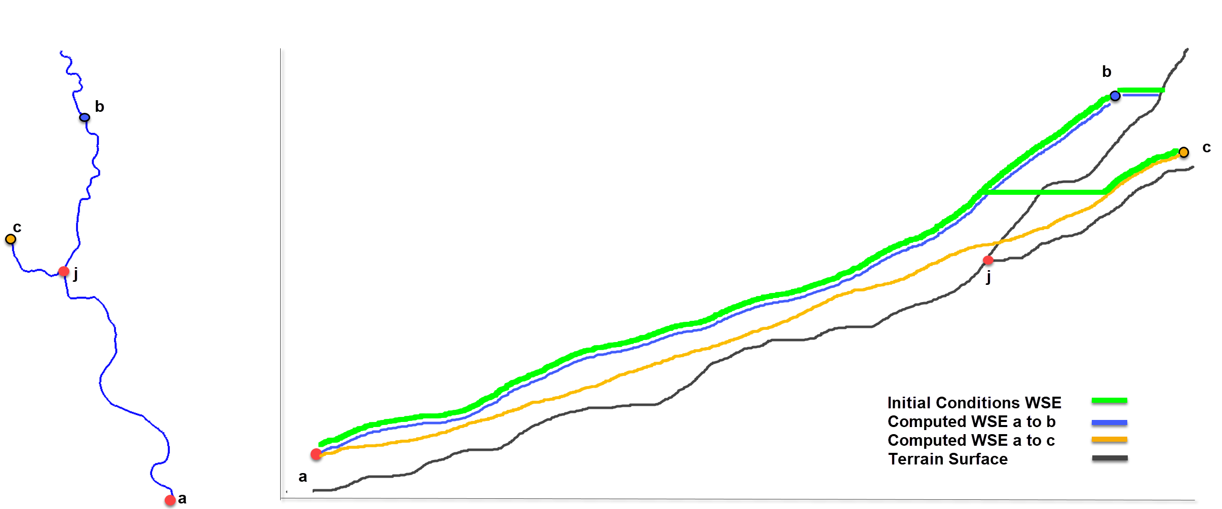
Using the unit flow width equation, HEC-RAS iteratively solves for a flow that meets the water surface (d, depth) at the upstream initial conditions point using the specified downstream boundary water surface elevation (downstream initial conditions point). For all locations between an IC Point and the Downstream IC Point, we solve for a water surface (assuming normal depth) based on the computed flow per unit width. Wherever a higher water surface is computed throughout the domain, the higher water surface is used. This will result in reasonable starting water surface for the 2D domain. If the initial water surface is not satisfactory, the warm up time step option can be used to settle down the water surface. An illustration of the computational procedure is shown below for a simple river system comprised of a river (a-b) with a tributary (j-c).
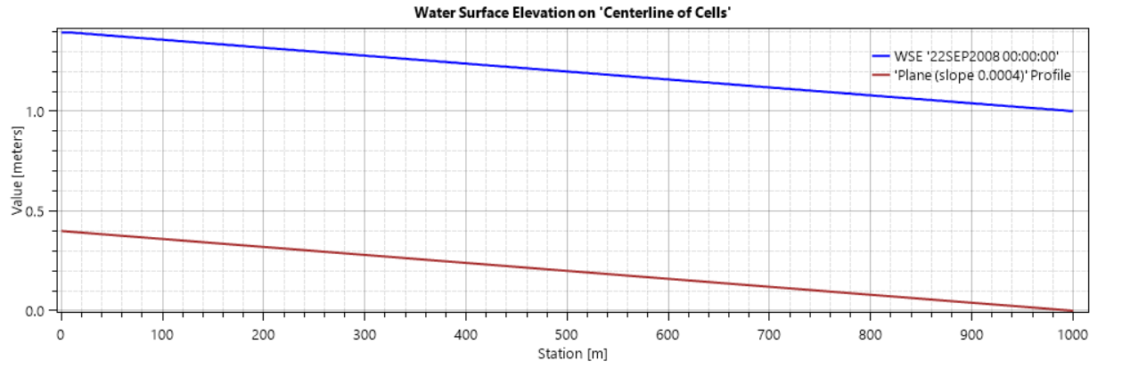
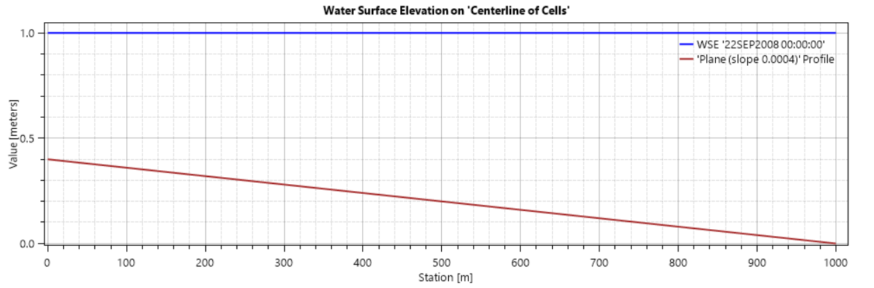
An example initial conditions for a planar surface 1000m long, set at a slope of 0.0004, with Manning's n value of 0.02 is shown in the figures below to illustrate the the computational process. The IC Points for the downstream water surface is computed to 1m depth.
Using a single IC Point at the downstream boundary results in a horizontal backwater.
Setting the Number of Warm Up Time Steps, holds flow constant, and results in the normal depth solution for the model domain where the water slope is equal to the bed slope.