Download PDF
Download page Creating an Infiltration Layer.
Creating an Infiltration Layer
RAS Mapper allows for the creation of an Infiltration layer. An Infiltration layer defines the Infiltration Method (Deficit Constant, SCS Curve Number, or Green and Ampt) that will be used for surface losses from a precipitation event. There are four different ways to generate an Infiltration layer in RAS Mapper: (1) using and existing RAS Land Cover layer, (2) using an existing RAS Soils layer, (3) using an intersection of a Land Cover layer and Soils layer, or (4) using a single classification shapefile layer. The approach used to create an infiltration layer for parameterization will depend on the selected infiltration method and data available.
Using a Land Cover and Soils Layer
When the Infiltration layer is created a complex table is created which cross references the Land Cover and Soils classifications from which the infiltration data can be parameterized. To create a complex Infiltration layer, select Map Layers | Create New RAS Layer | Infiltration Layer from Land Cover / Soils Layers menu item. The Infiltration Layer dialog show below will be invoked. The Infiltration Layer dialog allows the user to select the Infiltration Method, Land Cover Layer, and Soils Layer and provide the new Infiltration Layer Name and directory. Note, the user does not need to specify both a Land Cover layer and a Soils layer, this is a user option. However, for the SCS Curve Number Method, that is the best approach.
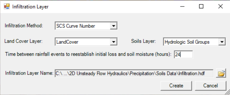
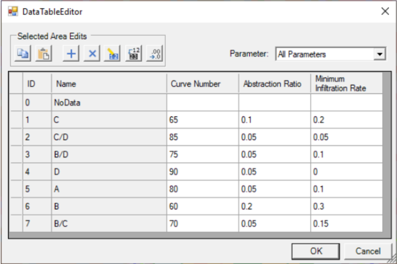
From the Infiltration Layer dialog (Figure 2-20), click the Create button to create a new raster layer that is the intersection of the land cover and soils layers. As shown in the figure below, the intersection of the layers can become quite complex, creating a Infiltration layer’s table with rows for each overlapping classification from the base layers. Depending on the infiltration method selection, additional columns for the required parameters will be provided. It is the user’s responsibility to fill out this table with an estimate for each of the parameters based on the Land Cover and the Soils data being used. In the example shown below, the user is required to enter an SCS Curve Number and an Abstraction Ratio (which defines initial losses). However, the Minimum Infiltration Rate field (Figure 2-21) is an optional parameter (which limits the infiltration rate). The Minimum Infiltration Rate field sets a threshold which will not allow the infiltration rate to be lower than the user entered value, even when the soil becomes saturated. This is not a standard feature of the SCS Curve number method, but an option added for HEC-RAS.
If the user has not entered any Percent Impervious data within the Land Cover data layer, then the CN values in the Infiltration layer’s table should reflect both pervious and impervious land surfaces within each Land Cover layer.

Using a Classification Shapefile Layer
To use a single classification layer, select Map Layers | Create New RAS Layer | Infiltration Layer from Shapefile | Method menu item. The Infiltration Layer dialog opens which will allow users to choose the shapefile of interest (click the Plus button to access the desired shapefile(s) from a browser window, and click Open to add the selected shapefile(s) to the Input Files table). Once the shapefile has been selected from the Input File table, select the unique classification name from the Name Field (like "Hydrologic Soils Group") to import the unique classification names (as shown in the figure below).
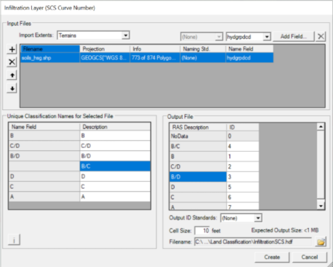
Click Create to close the Infiltration Layer dialog and import selected shapefile as a new Infiltration layer. Once the data has been imported, enter infiltration parameters by right clicking on the created Infiltration layer and selecting Edit Infiltration Data from the shortcut menu. A table will be provided with the infiltration parameters based on the Infiltration Method (Deficit Constant, SCS Curve Number, or Green and Ampt) selected.