Momentum Dispersion Stresses

Definition of Momentum Dispersion Stresses

The momentum dispersion stresses are defined as

1)	$\begin{array}{l}\displaystyle \boldsymbol{D} = D_{ij} = \frac{\rho}{h} \int_{z_b}^{z_s} \left( u_i(z) - U_i \right) \left( u_j(z) - U_j \right) dz\end{array}$

where

$\begin{array}{l}\boldsymbol{D} = D_{ij}\end{array}$ : dispersion stress tensor [M/L/T²]
$\begin{array}{l}U_i, U_j\end{array}$ : depth-averaged velocity components [L/T]
$\begin{array}{l}u_i(z), u_j(z)\end{array}$ : depth-varying velocity components [L/T]
$\begin{array}{l}\rho\end{array}$ : water density [M/L³]
$\begin{array}{l}h\end{array}$ : water depth [L]
$\begin{array}{l}z_b\end{array}$ : bed elevation [L]
$\begin{array}{l}z_s\end{array}$ : water surface elevation [L]

Streamwise Velocity Profiles

The streamwise component of the velocity can be assumed to have a power-law profile as

2)	$\begin{array}{l}\displaystyle \frac{u_s(\xi)}{\|\boldsymbol{U}\|} = \frac{m+1}{m} \xi^{1/m}\end{array}$

where

$\begin{array}{l}u_s(\xi)\end{array}$ : streamwise velocity [L/T]
$\begin{array}{l}\xi\end{array}$ : non-dimensional vertical coordinate [0, 1] [-]
$\begin{array}{l}m\end{array}$ : non-dimensional roughness parameter (approximately equal to 7) [-]
$\begin{array}{l}|\boldsymbol{U}|\end{array}$ : depth-averaged velocity magnitude [L/T]

The roughness parameter $\begin{array}{l}m\end{array}$ can be calculated from the Manning’s roughness coefficient by

3)	$\begin{array}{l}\displaystyle m = \frac{\kappa R^{1/6}}{g \sqrt{g}}\end{array}$

in which

$\begin{array}{l}\kappa\end{array}$ : von Karman constant [-]
$\begin{array}{l}n\end{array}$ : Manning’s roughness coefficient [T/L^1/3]
$\begin{array}{l}g\end{array}$ : gravity [L/T²]
$\begin{array}{l}R\end{array}$ : hydraulic radius [L]

An alternative velocity profile is a log-law profile given by

4)	$\begin{array}{l}\displaystyle \frac{u_s(\xi)}{\|\boldsymbol{U}\|} = \frac{ \ln( \xi / \xi_a)} {\ln(1 / \xi_a) - 1}\end{array}$

where

$\begin{array}{l}u_s(\xi)\end{array}$ : streamwise velocity [L/T]
$\begin{array}{l}\xi\end{array}$ : non-dimensional vertical coordinate [0, 1] [-]
$\begin{array}{l}\xi_a = z_a / h\end{array}$ : non-dimensional apparent roughness height [-]
$\begin{array}{l}z_a\end{array}$ : non-dimensional apparent roughness height [-]
$\begin{array}{l}h\end{array}$ : water depth [L]
$\begin{array}{l}|\boldsymbol{U}|\end{array}$ : depth-averaged velocity magnitude [L/T]

The apparent roughness height can be calculated from

5)	$\begin{array}{l}\displaystyle \xi_a = \frac{z_a}{h} = \exp(-1 - \kappa/ \sqrt{C_d}))\end{array}$

where

6)	$\begin{array}{l}\displaystyle C_d = \dfrac{g n^2}{R^{1/3}}\end{array}$

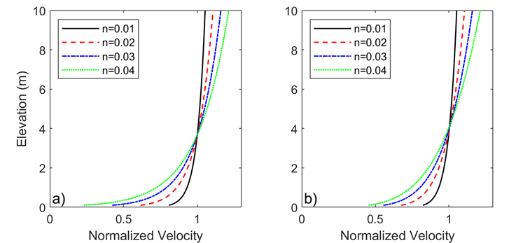
A comparison of Power-law and Logarithmic velocity profiles are shown in the figure below for various values of roughness coefficients. The velocity profiles are similar in the upper part of the water column but deviate in the lower part of the water column. In addition, the differences become more pronounced as the bottom roughness increases.

Transverse Velocity Profile

The transverse or spanwise velocity is approximated by the linear profile

7)	$\begin{array}{l}\displaystyle \frac{u_n(\xi)}{u_{ns}} = 2\xi - 1\end{array}$

where

$\begin{array}{l}u_n(\xi)\end{array}$ : transverse velocity [L/T]
$\begin{array}{l}\xi\end{array}$ : non-dimensional vertical coordinate [0, 1] [-]
$\begin{array}{l}u_{ns} = u_n(\xi = 1)\end{array}$ : transverse velocity at the surface [L/T]

Dispersion Stresses

Assuming power-law streamwise and linear transverse velocity profiles, the dispersion terms are given by

8)	$\begin{array}{l}\displaystyle D_{ij} = \dfrac{\rho U_i U_j}{m(m+2)} + \dfrac{U_i u_{nsj} + U_j u_{nsi} }{2m + 1} + \dfrac{\rho u_{nsi} u_{nsj} }{3}\end{array}$

Alternatively, assuming log-law streamwise and transverse velocity profiles, the dispersion terms are given by

9)	$\begin{array}{l}\displaystyle D_{ij} = \dfrac{\rho U_i U_j}{\left[ \ln(1/\xi_a) - 1 \right]^2} + \dfrac{U_i u_{nsj} + U_j u_{nsi} }{2 \left[ \ln(1/\xi_a) - 1 \right]} + \dfrac{\rho u_{nsi} u_{nsj} }{3}\end{array}$

In general, the logarithmic formulation produces larger dispersion coefficients. This is due to the sharp gradient of the velocity profile near the bed in the logarithmic velocity profile.