Introduction

The Navier-Stokes equations describe the motion of fluids in three dimensions. In the context of channel and flood modeling, further simplifications are imposed. One simplified set of equations is the Shallow Water (SW) equations. Incompressible flow, uniform density and hydrostatic pressure are assumed and the equations are Reynolds averaged so that turbulent motion is approximated using eddy viscosity. It is also assumed that the vertical length scale is much smaller than the horizontal length scales. As a consequence, the vertical velocity is small and pressure is hydrostatic, leading to the differential form of the SW equations derived in subsequent sections.

In some shallow flows the barotropic pressure gradient (gravity) term and the bottom friction terms are the dominant terms in the momentum equations and unsteady, advection, and viscous terms can be disregarded. The momentum equation then becomes the two dimensional form of the Diffusion Wave Approximation. Combining this equation with mass conservation yields a one equation model, known as the Diffusive Wave Approximation of the Shallow Water (DSW) equations.

Furthermore, in order to improve computation time, a sub-grid bathymetry approach can be used. The idea behind this approach is to use a relatively coarse computational grid and finer scale information about the underlying topography (Casulli, 2008). The mass conservation equation is discretized using a finite volume technique. The fine grid details are factored out as parameters representing multiple integrals over volumes and face areas. As a result, the transport of fluid mass accounts for the fine scale topography inside of each discrete cell. Since this idea relates only to the mass equation, it can be used independently of the version of the momentum equation. In the sections below, sub-grid bathymetry equations are derived in the context of both full Shallow Water (SW) equations and Diffusion Wave (DSW) equations.

In the Grid and Dual Grid subsequent section, the grid requirements are laid out and further notation is defined in order to develop a numerical solution algorithm.

The Numerical Methods section describes the details of the finite volume implementation. The numerical methods section also details the way in which the different terms of the equations are discretized and how the non-linear problem is transformed into a system of equations with variable coefficients. The global algorithm to solve the general unsteady problem is also explained in detail.

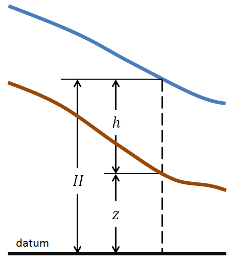
Through this document it will be assumed that the bottom surface elevation is given by $//<![CDATA[ \begin{array}{l}z_b(x,y)\end{array} //]]>$; the water depth is $//<![CDATA[ \begin{array}{l}h(x,y,t)\end{array} //]]>$; $//<![CDATA[ \begin{array}{l}z_s(x,y,t)\end{array} //]]>$ and the water surface elevation is: