Critical Creek - Example 1

Critical Creek is a steep river comprised of one reach entitled "Upper Reach." The purpose of this example is to demonstrate the procedure for performing a basic flow analysis on a single river reach. Additionally, the example will demonstrate the need for additional cross sections for a more accurate estimate of the energy losses and water surface elevations.

From the main HEC-RAS window, select File and then Open Project. Go to the directory in which you have installed the HEC-RAS example data sets. From the "Applications Guide\Example 1 – Critical Creek" subdirectory, select the project labeled "Critical Creek - Example 1." This will open the project and activate the following files:

Plan: "Existing Conditions Run"
Geometry: "Base Geometry Data"
Flow: "100 Year Profile"

Example 1 - Critical Creek.zip

Subcritical Flow Analysis

To begin, we will evaluate the river reach using the subcritical flow option.

Geometric Data

From the main program window, select Edit and then Geometric Data. This will activate the Geometric Data Editor and display the river system schematic, as shown in the figure below. As shown in the figure, the river name was entered as "Critical Creek," and the reach name was "Upper Reach." The reach was defined with 12 cross sections numbered 12 to 1, with cross section 12 being the most upstream cross section. These cross-section identifiers are only used by the program for placement of the cross sections in a numerical order, with the highest number being the most upstream section.

The cross section data were entered in the Cross Section Data Editor, which is activated by selecting the Cross Section icon on the Geometric Data Editor (as outlined in Chapter 6 of the User's Manual). Most of the 12 cross sections contain at least 50 pairs of X-Y coordinates, so the cross section data will not be shown here for brevity. The distances between the cross sections are as shown in the bottom figure below (The reach lengths for cross section 12 can be seen by using the scroll bars in the window.). This summary table can be viewed by selecting Tables and then Reach Lengths on the Geometric Data Editor.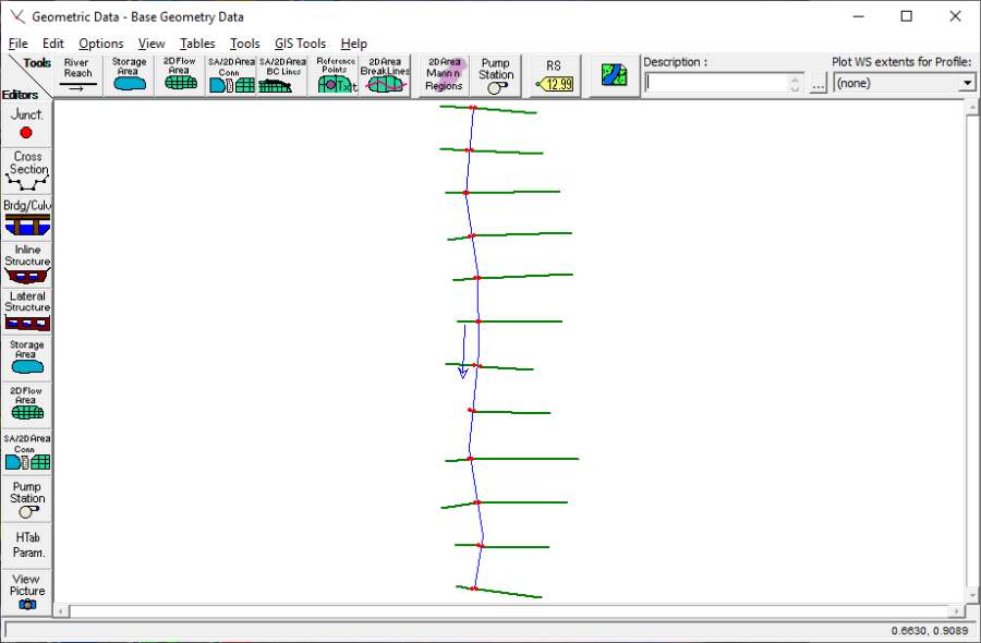



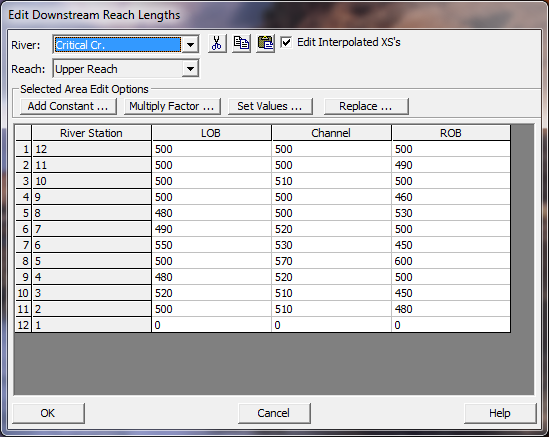
From the geometric data, it can be seen that most of the cross sections are spaced approximately 500 feet apart. The change in elevation from cross section 12 to cross-section 1 is approximately 56 feet along the river reach of 5700 feet. This yields a slope of approximately 0.01 ft/ft, which can be considered as a fairly steep slope. The remaining geometric data consists of Manning's n values of 0.10, 0.04, and 0.10 in the left overbank (LOB), main channel, and right overbank (ROB), respectively. Also, the coefficients of contraction and expansion are 0.10 and 0.30, respectively. After all the geometric data was entered, it was saved as the file "Base Geometry Data."

Flow Data

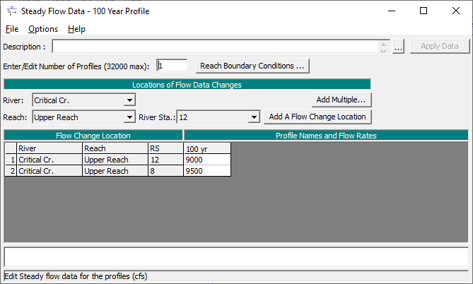
To enter the steady flow data, from the main program window Edit and then Steady Flow Data were selected. This activated the Steady Flow Data Editor, as shown in the figure below. For this steady flow analysis, the one percent chance flow profile was analyzed. A flow of 9000 cfs was used at the upstream end of the reach at section 12 and a flow change to 9500 cfs was used at section 8 to account for a tributary inflow into the main river reach. This flow change location was entered by selecting the river, reach, river station, and then pressing the Add A Flow Change Location button. Then, the table in the central portion of the editor added the row for river station 8. Finally, the profile name was changed from the default heading of "PF#1" to "100 yr." The change to the profile label was made by selecting Edit Profile Names from the Options menu and typing in the new name.

Next, the Reach Boundary Conditions button located at the top of the Steady Flow Data Editor was selected. The reach was analyzed for subcritical flow with a downstream normal depth boundary condition of S = 0.01 ft/ft. This value was estimated as the average slope of the channel near the downstream boundary. For a subcritical flow analysis, boundary conditions must be set at the downstream end(s) of the river system. After all of the flow data was entered, it was saved as the file "100 Year Profile."

Steady Flow Analysis

To perform the steady flow analysis, from the main program window Run and then Steady Flow Analysis were selected. This activated the Steady Flow Analysis Window as shown in the figure below. Before performing the steady flow analysis, Options and then Critical Depth Output Option were selected. The option Critical Always Calculated was chosen to have critical depth calculated at all locations. This will enable the critical depth to be plotted at all locations on the profile when the results are analyzed. Next, the Flow Regime was selected as "Subcritical". The geometry file was selected as "Base Geometry Data," and the flow file was selected as "100 Year Profile". The plan was then saved as "Existing Conditions", with a short ID of "Exist Cond". Finally, the steady flow analysis was performed by selecting COMPUTE from the Steady Flow Analysis window.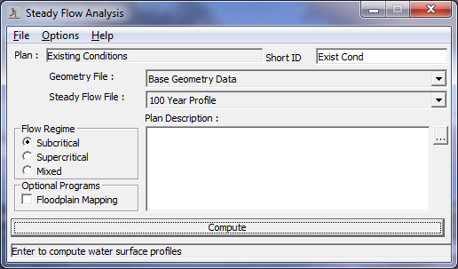

Subcritical Flow Output Review

As an initial view of the steady flow analysis output, from the main program window View and then Water Surface Profiles were selected. This activated the water surface profile as shown in the figure below. From the Options menu, the Variables of water surface, energy, and critical depth, were chosen to be plotted.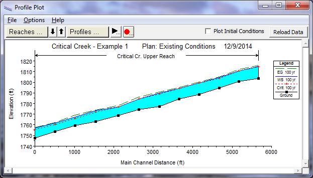

From this profile, it can be seen that the water surface appears to approach or is equal to the critical depth at several locations. For example, from section 12 through 8, the water surface appears to coincide with the critical depth. This implies that the program may have had some difficulty in determining a subcritical flow value in this region, or perhaps the actual value of the flow depth is in the supercritical flow regime. To investigate this further, a closer review of the output needs to be performed. This can be accomplished by reviewing the output at each of the cross sections in either graphical or tabular form, and by viewing the summary of Errors, Warnings and Notes.

First, a review of the output at each cross section will be performed. From the main program window, select View, Detailed Output Tables, Type, and then Cross Section. Selection of cross section 12 should result in the display as shown in the figure below. At the bottom of the table is a box that displays any errors, warnings, or notes that are specific to that cross section. For this example, there are several warning messages at cross section 12. The first warning is that the velocity head has changed by more than 0.5 feet and that this may indicate the need for additional cross sections. To explain this message, it is important to remember that for a subcritical flow analysis, the program starts at the downstream end of the reach and works upstream. After the program computed the water surface elevation for the 11th cross section, it moved to the 12th cross section. When the program computed the water surface elevation for the 12th cross section, the difference in the velocity head from the 11th to the 12th cross section was greater than 0.5 feet. This implies that there was a significant change in the average velocity from section 11 to section 12. This change in velocity could be reflecting the fact that the shape of the cross section is changing dramatically and causing the flow area to be contracting or expanding, or that a significant change in slope occurred. In order to model this change more effectively, additional cross sections should be supplied in the region of the contraction or expansion. This will allow the program to better calculate the energy losses in this region and compute a more accurate water surface profile.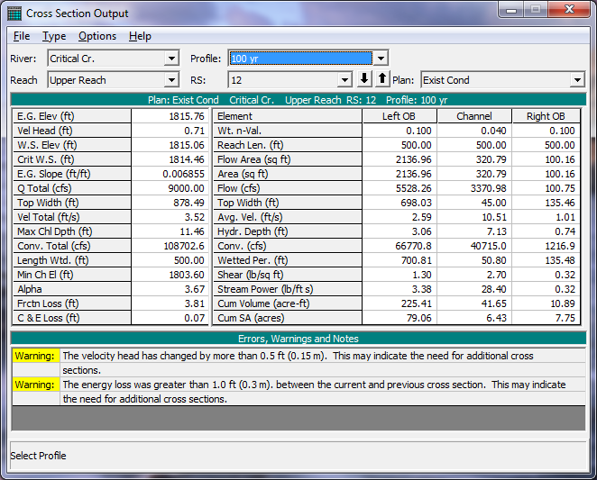

The second warning at cross section 12 states that the energy loss was greater than 1.0 feet between the current cross section (#12) and the previous cross section (#11). This warning also indicates the possible need for additional cross sections. This is due to the fact that the rate of energy loss is usually not linear. However, the program uses, as a default, an average conveyance equation to determine the energy losses. Therefore, if the cross sections are too far apart, an appropriate energy loss will not be determined between the two cross sections. (The user may select alternate methods to compute the average friction slope. Further discussion of user specified friction loss formulation is discussed in Chapter 4 of the Hydraulic Reference Manual.)

A review of other cross sections reveals the same and additional warnings. To review the errors, notes, and warnings for all of the cross sections, select Summary Errors, Warnings, and Notes from the View menu on the main program window. A portion of the summary table is shown in the figure below.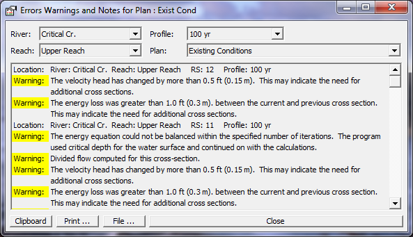

The additional warnings and notes that are listed in the summary table are described as follows.

Warning - The energy equation could not be balanced within the specified number of iterations. The program used critical depth for the water surface and continued on with the calculations.

This warning implies that during the computation of the upstream water surface elevation, the program could not compute enough energy losses to provide for a subcritical flow depth at the upstream cross section. Therefore, the program defaulted to critical depth and continued on with the analysis.

Warning - The energy equation could not be balanced within the specified number of iterations. The program used critical depth for the water surface and continued on with the calculations.

After the flow depth was calculated for the cross section, the program determined that the flow was occurring in more than one portion of the cross section. For example, this warning occurred at river station # 10 and the plot of this cross section is shown in the figure below. From the figure, it can be seen that at approximately an X-coordinate of 800, there exists a large vertical land mass. During this output analysis, it must be determined whether or not the water can actually be flowing on both sides of the land mass at this flow rate. Since the main channel is on the right side of the central land mass, could the water be flowing on the left side or should all of the flow be contained to the right side of the land mass? By default, the program will consider that the water can flow on both sides of the land mass. If this is not correct, then the modeler needs to take additional action.

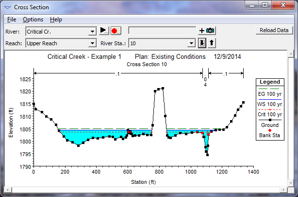
Additional action can be one of two procedures. First, if the existing scenario is not feasible, then the water on the left side may be considered as an ineffective flow area, where the water is accounted for volumetrically but it is not considered in the conveyance determination until a maximum elevation is reached. Secondly, if all of the flow should be occurring only on the right side of the land mass, then the land mass could be considered as a levee. By defining the central vertical land mass as a levee, the program will not permit a flow onto the left side of the levee until the flow depth overtops the levee.

For further discussion on ineffective flow areas and levees, refer to Chapter 6 of the User's Manual and Chapter 3 of the Hydraulic Reference Manual.

• Warning - During the standard step iterations, when the assumed water surface was set equal to critical depth, the calculated water surface came back below critical depth. This indicates that there is not a valid subcritical answer. The program defaulted to critical depth. This warning is issued when a subcritical flow analysis is being performed but the program could not determine a subcritical flow depth at the specified cross section. As the program is attempting to determine the upstream depth, it is using an iterative technique to solve the energy equation. During the iterations, the program tried critical depth as a possible solution, which resulted in a flow depth less than critical. Since this is not possible in a subcritical analysis, the program defaulted to using critical depth at this cross section and continued on with the analysis. This error is often associated with too long of a reach length between cross sections or misrepresentation of the effective flow area of the cross section.
• Warning - The parabolic search method failed to converge on critical depth. The program will try the cross section slice/secant method to find critical depth. This message appears if the program was required to calculate the critical depth and had difficulty in determining the critical depth at the cross section. The program has two methods for determining critical depth: a parabolic method and a secant method. The parabolic method is the default method (this can be changed by the user) because this method is faster and most cross sections have only one minimum energy point. However, for cross sections with large, flat over banks, there can exist more than one minimum energy point. For further discussion, refer to the section Critical Depth Determination in Chapter 2 of the Hydraulic Reference Manual.
• Note - Multiple critical depths were found at this location. The critical depth with the lowest, valid, water surface was used. This note appears when the program was required to determine the critical depth and accompanies the use of the secant method in the determination of the critical depth (as described in the previous warning message). This note prompts the user to examine closer the critical depth that was determined to ensure that the program supplied a valid answer. For further discussion, refer to the section Critical Depth Determination in Chapter 2 of the Hydraulic Reference Manual.

• Warning - The conveyance ratio (upstream conveyance divided by downstream conveyance) is less than 0.7 or greater than 1.4. This may indicate the need for additional cross sections. The conveyance of the cross section, K, is defined by:

  $$//<![CDATA[ \begin{array}{l}\displaystyle K = \frac{1.486}{n} AR^\frac{2}{3}\end{array} //]]>$$

If the n values for two subsequent cross sections are approximately the same, it can be seen that the ratio of the two conveyances is primarily a function of the cross sectional area. If this ratio differs by more than 30%, then this warning will be issued. This warning implies that the cross sectional areas are changing dramatically between the two sections and additional cross sections should be supplied for the program to be able to more accurately compute the water surface elevation.

In summary, these warnings and notes are intended to inform the user that potential problems may exist at the specified cross sections. It is important to note that the user does not have to eliminate all the warning messages. However, it is up to the user to determine whether or not these warnings require additional action for the analysis.

Mixed Flow Analysis

Upon reviewing the profile plot and the summary of errors, warnings, and notes from the subcritical flow analysis, it was determined that additional cross-section information was required. Additionally, since the program defaulted to critical depth at various locations along the river reach and could not provide a subcritical answer at several locations, a subsequent analysis in the mixed flow regime was performed. A mixed flow analysis will provide results in both the subcritical and supercritical flow regimes.

Modification of Existing Geometry

Before performing the mixed flow regime analysis, the existing geometry was modified by adding additional cross sections. To obtain the additional cross section information, the modeler should use surveyed cross section data whenever possible. If this data are not available, then the cross section interpolation method within the HEC-RAS program can be used. However, this method is not intended to be a replacement for actual field data. The modeler should review all interpolated cross sections because they are based on a linear transition between the input sections. Whenever possible, use topographic maps for assistance in evaluating whether or not the interpolated cross sections are adequate. The modeler is referred to the discussions in Chapter 6 of the User's Manual and Chapter 4 of the Hydraulic Reference Manual for additional information on cross section interpolation.

To obtain additional cross sections for this example, the interpolation routines were used. From the Geometric Data Editor, Tools and then XS Interpolation was selected. The initial type of interpolation was Within a Reach. The interpolation was started at cross section 12 and ended at cross section 1. The maximum distance was set to be 150 feet (This value can be changed later by the modeler to develop any number of cross sections desired.). Finally, Interpolate XS's was selected. When the computations were completed, the window was closed. At this point, the modeler can view each cross-section individually or the interpolated sections can be viewed between the original sections. The latter option is accomplished by selecting Tools, XS Interpolation, and then Between 2 Xs's. The up and down arrows are used to toggle up and down the river reach, while viewing the interpolated cross sections. When the upper river station is selected to be 11 (the lower station will automatically be 10), the interpolation shown in the figure below should appear.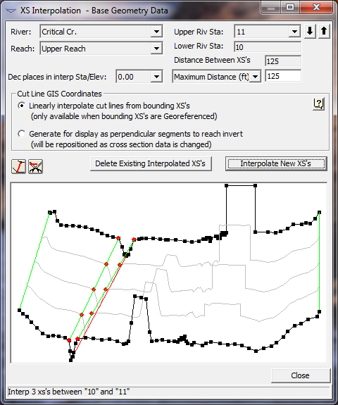

The interpolation was adequate for the right overbank and the main channel. However, the interpolation in the left overbank failed to connect the two existing high ground areas. These two high ground areas could be representing a levee or some natural existing feature. Therefore, Del Interp was selected to delete the interpolation. (This only deleted the interpolation between cross sections 11 and 10.) Then, the two high points and the low points of the high ground areas were connected with user supplied master cords. This was accomplished by selecting the Master Cord button and connecting the points where the master cords should be located. Finally, a maximum distance of 150 feet was entered between cross sections and Interpolate was selected. The final interpolation appeared as is shown in the following figure.

The modeler should now go through all of the interpolated cross sections and determine that the interpolation procedure adequately produced cross sections that depict the actual geometry. When completed, the geometric data was saved as the new file name "Base Geometry + Interpolated." This allowed the original data to be unaltered and available for future reference.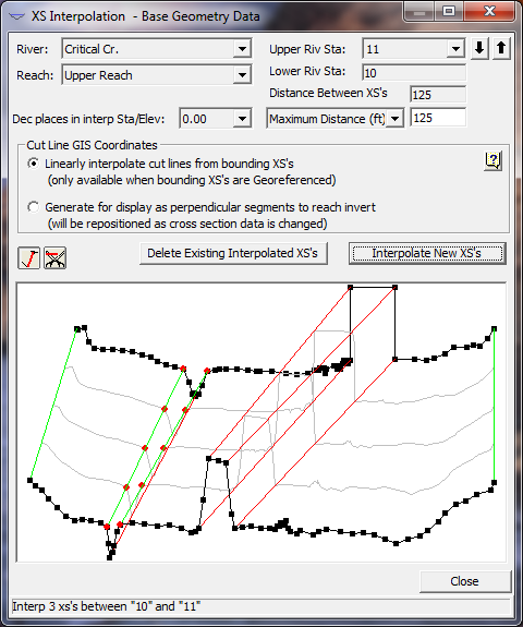

Flow Data

At this point, with the additional cross sections, the modeler can perform a flow analysis with subcritical flow as was performed previously and compare the results with the previously obtained data. However, for the purposes of this example, an upstream boundary condition was added and then a mixed flow regime analysis was performed. Since a mixed flow analysis (subcritical and supercritical flow possibilities) was selected, an upstream boundary condition was required. From the main program window, Edit and then Steady Flow Data were selected. Then the Boundary Conditions button was chosen and a normal depth boundary condition was entered at the upstream end of the reach. A slope of 0.01 ft/ft as the approximate slope of the channel at section 12 was used. Finally, the flow data was saved as a new file name. This will allow the modeler to recall the original data when necessary. For this example, the new flow data file was called "100 YR Profile - Up and Down Bndry." that includes the changes previously mentioned.

Mixed Flow Analysis

To perform the mixed flow analysis, from the main program window Run and Steady Flow Analysis were selected. The flow regime was selected to be "Mixed," the geometry file was chosen as "Base Geometry + Interpolated," and the steady flow file as "100 YR Profile - Up and Down Bndry." The Short ID was entered as "Modified Geo," and then File and Save Plan As were selected and a new name for this plan was entered as "Modified Geometry Conditions". This plan will then associate the geometry, flow data, and output file for the changes that were made. Finally, COMPUTE was selected to perform the steady flow analysis.

Review of Mixed Flow Output

As before, the modeler needs to review all of the output, which includes the profile as well as the channel cross sections both graphically and in tabular form. Also, the list of errors, warning, and notes should be reviewed. The modeler then needs to determine whether additional action needs to be taken to perform a subsequent analysis. For example, additional cross sections may still need to be provided between sections in the reach. The modeler may also consider to use additional flow profiles during the next analysis. The modeler should review all of the output data and make changes where they are deemed appropriate.

For this analysis, the resulting profile plot is shown in the figure below. From this figure, it can be seen that the flow depths occur in both the subcritical and supercritical flow regimes. (The user can use the zoom feature under the Options menu in the program. This can imply that the geometry of the river reach and the selected flows are producing subcritical and supercritical flow results for the reach.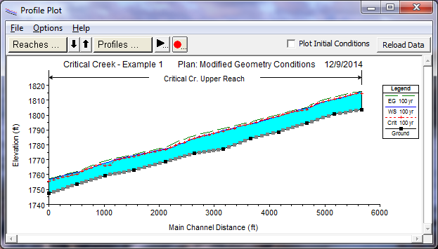

To investigate this further, the results will be viewed in tabular form. From the main program window, View, Profile Summary Tables, Std. Tables, and then Standard Table 1 were selected. This table for the mixed flow analysis is shown in the Standard Table 1 (shown below). The table columns show the default settings of river, reach, river station, total flow, minimum channel elevation, water surface elevation, etc. The meanings of the headings are described in a box at the bottom of the table. By selecting a cell in any column, the definition of the heading will appear in the box for that column.

From the Standard Table 1, the water surface elevations and critical water surface elevations can be compared. The values at river station 11.2* show that the flow is supercritical at this cross section since the water surface is at an elevation of 1811.29 ft and the critical water surface elevation is 1811.46 ft. Additionally, it can be seen that the flow at river station 11.0 is subcritical. (Note: the asterisks "*" denote that the cross sections were interpolated.) By selecting the Cross Section type table (as performed above), and toggling to river station 11.0, a note appears at the bottom of the table indicating that a hydraulic jump occurred between this cross section and the previous upstream cross section. These results are showing that the flow is both subcritical and supercritical in this reach. The user can continue this process of reviewing the warnings, notes, profile plot, profile tables, and cross section tables to determine if additional cross sections are required.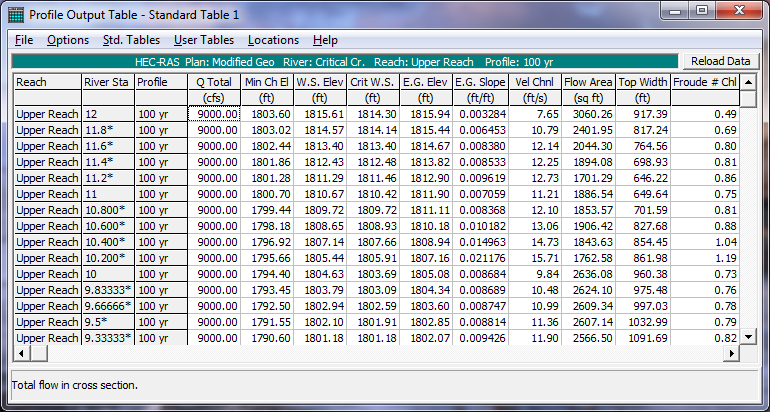

Critical Creek Summary

Initially, the river reach was analyzed using the existing geometric data and a subcritical flow regime. Upon analysis of the results, it was determined that additional cross-section data were needed and that there might be supercritical flow within the reach. Additional cross sections were then added by interpolation and the reach was subsequently analyzed using the mixed flow regime method. Review of the mixed flow analysis output showed the existence of both subcritical and supercritical flow within the reach. This exhibits that the river reach is set on a slope that will produce a water surface around the critical depth for the given flow and cross section data. Therefore, a completely subcritical or supercritical profile is not possible.