Ice-Covered River - Example 14

This example, which demonstrates the analysis of an ice-covered river, focuses on describing a river ice cover and a river ice jam in HEC-RAS. The water surface elevations resulting from the presence of an ice cover or an ice jam can then be compared to the equivalent open water case. The estimated ice jam thicknesses can also be compared to the measured jam thickness Beltaos, S., and W.J. Moody (1986) Measurements of the Configuration of a Breakup Jam. NWRI Contribution 86-123. National Water Research Institute, Canada Center for Inland Waters, Burlington, Ontario, Canada L7R 4A6.

An ice cover changes the effective channel geometry. This means that separate geometry files must be created for the open water case, the ice cover case, and the ice jam case. The best approach is to create a separate plan for each. See Chapter 5 of the User's Manual and Example 7 of the Application Manual for a further discussion on working with projects and a discussion of the files that constitute a plan.

The data for this example were entered in metric units. To review the data files for this example, from the main HEC-RAS window, select File and then Open Project. Go to the directory in which you have installed the HEC-RAS example data sets. From the "Applications Guide\Example 14 – Ice Covered River" subdirectory, select the project labeled "Thames River Ice Jam -Example 14." This will open the project and activate the following files:

Plan: "Thames River Open Water Analysis"
Geometry: "Thames River Open Water Data"
Flow: "Estimated Thames River Flow"

Example 14 - Ice Covered River.zip

Open Water Analysis

Three geometry files are created for this project, and all are based on the same channel geometry and channel properties. Only the ice cover description varies among plans.

Open Water Geometry

A geometry file was created that modeled the existing conditions for a reach of the Thames River. This reach is a natural channel where an ice jam occurred. To view the river system schematic, select Edit and then Geometric Data from the main program window. This will activate the Geometric Data Editor and display the river system schematic. This is a very simple schematic with a single straight channel. The river is the Thames River and it has only a single reach: Ice Jam Section.

The river reach is defined by 22 river stations. The user can view the geometric data for each river station by selecting the Cross Section icon from the Geometric Data Editor. The data for each river station comprises X and Y coordinates, downstream reach lengths, Manning's n values, main channel bank stations, and contraction and expansion coefficients. There was no out-of-channel flow during the ice jam event. As a result, overbank areas are not included. There are no structures in this section of channel.

After all geometric data were entered, the geometry file was saved using the title "Thames River Open Water Data."

Steady Flow Data

Next, the steady flow data file was created by selecting Edit and Steady Flow Data from the main program window. This activated the Steady Flow Data Editor. The profile selected to be analyzed corresponds to the estimated flow during the ice jam event. The flow value of 261 cubic meters per second (CMS) was entered at river station 42000 (the upstream river station), and a known downstream water surface elevation of 177.64 meters was entered by selecting the Boundary Conditions icon. Next, the observed water surface elevations during the ice jam event were entered by selecting Options and then Observed WS using the Steady Flow Data Editor. The observed water levels at nine river stations were then entered. After all steady flow data were entered, the steady flow file was saved using the title "Estimated Thames River Flow."

Open Water Plan

After the geometric data and steady flow data were entered and saved, a plan entitled "Thames River Open Water Analysis" was created by first selecting Run and then Steady Flow Analysis from the main program window. The plan itself was created in the Steady Flow Analysis Window. Again, see Chapter 5 of the User's Manual and Example 7 of the Application Manual for further discussion of the files that constitute a plan. A subcritical analysis was chosen as the Flow Regime and then File and Save Plan As were selected. The title "Thames River Open Water Analysis" was entered and the OK button selected. The Short ID for this plan was set as "open_water."

After the plan was saved, the Compute button was selected to execute the program. Note that the calculation required only one iteration to solve the steady flow equations for the entire channel.

Open Water Output

The rather straightforward open water output will not be reviewed here. Note that the water surface elevations calculated assuming open water do not match the observed ice jam elevations at all, as would be expected.

Ice Cover Analysis

To analyze the case of a continuous ice cover, an ice cover with a constant thickness and roughness will be placed on the channel. To do this analysis, the geometry file was modified to reflect the presence of the ice cover. Then a new plan was created with the new geometry file and the original steady flow file. This procedure is outlined below.

Ice Cover Geometry

To add the ice cover, the geometry file "Thames River Open Water Data" was activated. At this point, the modeler has the option of entering the ice cover properties cross section by cross section, by selecting the Cross Section icon from the Geometric Data Editor, or by selecting Tables and then Ice Cover from the Geometric Data Editor. In this case, the Tables option was used. First, the Chan Ice Thickness column was highlighted by dragging the mouse over the entire length of the column. Then the Set Values icon was clicked and the value of 0.5 meters was entered. This value corresponds to a reasonable, end-of-winter ice thickness that results from thermal growth. It was not necessary to enter ice thicknesses for either overbank, as no overbank areas were included in this simulation. In a similar way, the Manning's n value was set for the channel ice cover by entering the Manning n value in the Chan ice Mann n column using the Set Values icon. In this case a value of 0.03 was used, typical for a floating smooth ice cover.

After all of the ice cover data were entered, the geometry file was saved using the Geometric Data editor by selecting File and the Save Geometry Data As. The title entered was "Thames River Ice Cover Data."

Steady Flow Data

The steady flow analysis of the ice-covered channel will use the same flow data used in the open water geometry. Therefore, there were no adjustments made to the steady flow data in the file "Estimated Thames River Flow."

Ice Cover Plan

A new plan was created from the geometry file with the ice cover and the steady flow data file. This plan was created by first selecting Run and then Steady Flow Analysis from the main program window. The plan itself was created in the Steady Flow Analysis Window. A Short ID for this plan was set as "ice_covered." The geometry file "Thames River Ice Cover Data" and the steady flow file "Estimated Thames River Flow" were selected by using the down arrows on the right side of the window. A subcritical analysis was chosen as the Flow Regime, and then File and Save Plan As were selected. The title "Thames River Ice Cover Analysis" was entered and the OK button selected. After the plan was saved, the Compute button was selected to execute the program. Note that the calculation required only one iteration to solve the steady flow equations for the entire channel.

Ice Cover Output

The rather straightforward ice-covered channel output will not be reviewed here. It can be noted that the water surface elevations calculated by assuming an ice cover do not match the observed ice jam elevations at all, as would be expected.

Ice Jam Analysis

To analyze the case of an ice jam, an ice jam simulation will be selected for the channel. To do this analysis, the geometry file was modified to reflect the presence of the ice jam. Then a new plan was created with the new geometry file and the original steady flow file. This procedure is outlined below.

Ice Jam Geometry

To add the ice jam, the geometry file "Thames River Open Water Data" was activated. At this point, the modeler has the option of entering the ice jam properties cross section by cross section, by selecting the Cross Section icon from the Geometric Data Editor, or by selecting Tables and then Ice Cover from the Geometric Data Editor. In this case, the Tables option was used. First, the Chan Ice Thickness column was highlighted by dragging the mouse over the entire length of the column. Then the Set Values icon was clicked and the thickness value of 0.5 meter was entered. In fact, HEC-RAS will estimate the jam thickness, but these entered values will represent the minimum allowable ice thickness in the jam. This thickness was selected on the basis of field observations, which showed that no cross section had a minimum thickness less than 0.5 m. This minimum jam thickness value will vary from river reach to river reach, and it is probably worth trying several minimum jam thickness values at any location. Next, it was necessary to indicate to HEC-RAS that this simulation should be treated as an ice jam and not an ice cover with fixed thickness. This is done in the Ice Jam Chan column of the Ice Cover Table by changing the default value of n (no) to y (yes) for each river station where the ice jam is thought to have occurred. (Note that this must be done for each river section individually, as the Set Values icon will not work for yes/no input.) In this case, it is not necessary to change the default values of n in the column Ice Jam OB, as there is no overbank flow.

It is necessary to fix the ice thickness in the sections immediately upstream and downstream of the jam, because a cross section with known ice thickness is required at the upstream and downstream limits of the jam. In this case, a thickness of 0.5 m was set for the upstream and downstream river station of the Ice Jam Reach, and the value in the Ice Jam Chan column was set to n for these two river stations. It is important to remember that for every ice jam, there must be an n set in the Ice Jam Chan column immediately upstream and downstream of the jam.

The nominal Manning's n value was set for the channel ice cover by entering the Manning n value in the Chan ice Mann n column using the Set Values icon. However, in this case, it is desired that HEC-RAS estimate the Manning's n of the jam using the procedure outlined in the Hydraulic Reference Manual. It is necessary to indicate to HEC-RAS that this simulation should estimate the Manning's n of the ice jam and not use the value entered in the Chan ice Mann n column. This is done in the Fixed Mann n column by changing the default value of y to n. The default value of y was entered for the upstream and downstream river stations of the Ice Jam Reach, because these stations are considered to have a known roughness as well as a known thickness.

The other parameters, which describe the ice jam material properties, such as the friction angle, porosity, and stress ratio, were all left at their default values. In most cases, it will not be necessary to modify these values from their default values. After all of the ice cover data were entered, the geometry file was saved using the Geometric Data editor by selecting File and the Save Geometry Data As. The title entered was "Thames River Ice Jam Data."

Steady Flow Data

The steady flow analysis of the ice jam will use the same flow data as the open water geometry. Therefore there were no adjustments made to the steady flow data in the file "Estimated Thames River Flow."

Ice Jam Plan

A new plan was created from the geometry file with the ice cover and the steady flow data file. This plan was created by first selecting Simulate and then Steady Flow Analysis from the main program window. The plan itself was created in the Steady Flow Analysis Window. A Short ID for this plan was set as "ice_jam." The geometry file "Thames River Ice Jam Data" and the steady flow file "Estimated Thames River Flow" were selected by using the down arrows on the right side of the window. A subcritical analysis was chosen as the Flow Regime and then File and Save Plan As were selected. The title "Thames River Ice Jam Analysis" was entered and the OK button selected. After the plan was saved, the Compute button was selected to execute the program. Note that the calculation required a number of iterations to solve the steady flow equations and the ice jam force balance equation for the entire reach. The calculations iterate until the calculated jam thicknesses and water surface elevations converge to a constant value within the minimum tolerances. See the Hydraulic Reference Manual section on ice jam calculations for more information on the convergence criteria.

Ice Jam Output

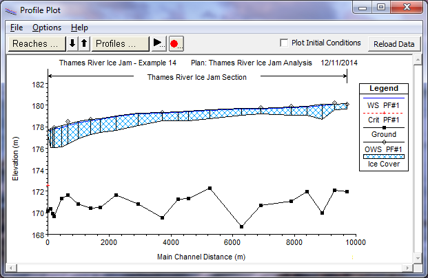
The ice jam results are shown in a graphical profile plot in the figure below. The calculated ice jam thickness along the channel, the water surface elevations, and the observed water surface elevations at selected cross sections are shown. Note that the calculated ice jam water surface elevations match the observed water surface elevations reasonably well.

Comparison of Open Water, Ice Cover, and Ice Jam Results

To compare the output from the three plans, the user can view the results graphically and in tabular format. In the interest of brevity, not all the graphical plots that are available will be illustrated here.

Profile Plot

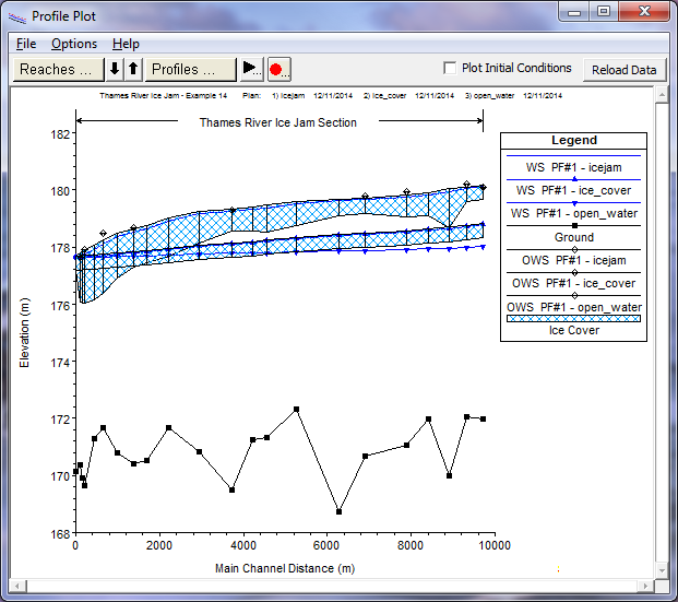
At this point, the results of all three plans can be compared. The profile plot of the ice jam, the river ice cover, and the open water results can be seen in the figure below It is also possible to graphically display comparisons of the results in Cross Section Plots, and X-Y-Z- Perspective Plots.

Ice Table

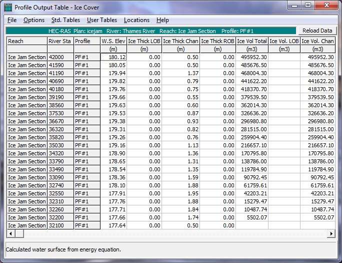
In addition to graphical displays, it is possible to compare the output in tabular form. From the main program window, select View and then Profile Summary Table. By selecting Ice Cover under the Std. Tables menu, a table with the ice results will be shown. This table includes the ice thickness (if any) at each river section, the calculated water surface elevations at each section, the cumulative ice volume in the channel and overbanks, and the calculated weighted Manning's n at each section. This table can be used to compare the results from each plan. An example ice table is shown in the figure below.