Looped Network - Example 8

This example was performed to demonstrate the analysis of a river reach that contains a loop. The loop is caused by a split in the main channel that forms two streams which join back together.

The focus of this example is on the development of the looped network and the balancing of the flows through each branch of the loop. The stream junctions will be discussed briefly; however, a more detailed discussion of stream junctions can be found in Example 10. Note: Since this example was developed, we have added the ability to have the program optimize the flow split at junctions for you. Example application 15 shows how to use the split flow optimization routine.

To review the data files for this example, from the main HEC-RAS window, select File and then Open Project. Go to the directory in which you have installed the HEC-RAS example data sets. From the "Applications Guide\Example 8 – Looped Network" subdirectory, select the project labeled "Looped Network - Example 8." This will open the project and activate the following files:

Plan: "Looped Plan"
Geometry:"Looped Geometry"
Flow: "10, 50, and 100 year flow events"

Example 8 - Looped Network.zip

Geometric Data

The geometric data for this example consists of the river system schematic, the cross section data, and the stream junction data. Each of these components are discussed below.

River System Schematic

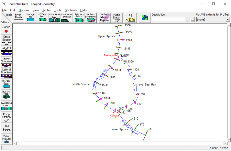
To view the river system schematic, from the main program window select Edit and then Geometric Data. This will activate the Geometric Data Editor and display the river system schematic as shown in the figure below. The schematic shows the layout of the two rivers. Spruce Creek is broken into three river reaches: Upper Spruce Creek, Middle Spruce Creek, Lower Spruce Creek. Bear Run is left as a single river reach. The flow in Upper Spruce Creek splits at Tusseyville to form Bear Run and Middle Spruce Creek. Bear Run is approximately 1500 feet in length and Middle Spruce Creek is approximately 1000 feet long. These two streams then join at Coburn to form Lower Spruce Creek.

Cross Section Data

After the river reaches were sketched to form the river system schematic, the cross section data were entered. The data were entered by selecting the Cross Section icon from the Geometric Data Editor. For each cross section, the geometric data consisted of the: X-Y coordinates, downstream reach lengths, Manning's n values, main channel bank stations, the contraction and expansion coefficients, and, if applicable, left or right levees.

After all of the geometric data were entered, File and then Save Geometry Data As were selected from the Geometric Data Editor. The title "Looped Geometry" was entered and the OK button selected. This was the only geometry file for this example.

Stream Junction Data

The final geometric component was the data for the stream junction. These data were entered by selecting the Junction icon on the Geometric Data Editor. This caused the Junction Data Editor to appear as shown in the figure below. First, the data for the junction at Tusseyville was entered by selecting the appropriate Junction Name at the top of the editor. Then a Description was entered as "Spruce Creek Split."

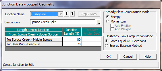
The next piece of information required was the Length Across Junction. These are the distances from the downstream river station of Upper Spruce to the upstream river stations of Middle Spruce and Bear Run. In general, the cross sections that bound a junction should be placed as close to the junction as possible. This will allow for a more accurate calculation of the energy losses across the junction. These values were entered as 80 and 70 feet, for the distances to Middle Spruce and Bear Run, respectively.

The last item in the junction editor is the computation mode. Either the Energy or the Momentum method must be selected. The energy method (the default method) uses a standard step procedure to determine the water surface across the junction. The momentum method takes into account the angle of the tributaries to evaluate the forces associated with the tributary flows. For this example, the flow velocities were low and the influence of the tributary angle was considered insignificant. Therefore, the energy method was selected for the analysis. For a further discussion on stream junctions, the user is referred to example 10 and to chapter 4 of the Hydraulic Reference Manual.

After the data were entered for the Tusseyville Junction, the Apply Data button was selected. The down arrow adjacent to the Junction Name was depressed to activate the second junction at Coburn. At this junction, the description "Confluence of Bear Run and Middle Spruce" was entered. Next, a length of 70 feet was entered from Bear Run to Lower Spruce and 85 feet for the distance from Middle Spruce to Lower Spruce. Again, the energy method was selected and the Apply Data button was chosen before closing the junction editor.

Steady Flow Data

The steady flow data were entered next. These data consisted of the profile data and the boundary conditions. Each of these items is discussed as follows.

Profile Data

To enter the steady flow data, the Steady Flow Data Editor was activated from the main program window by selecting Edit and then Steady Flow Data. This opened the editor as shown in the figure below. On the first line of the editor, the number of profiles was chosen to be 3. These profiles will represent the 10, 50, and 100 - year flow events. When the number of profiles is entered, the table expands to provide a column for each profile.

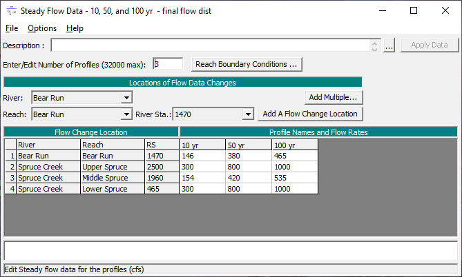
To enter the flow data, a flow value must be entered at the upstream end of each reach. The program will consider the flow rate to be constant throughout the reach unless a change in flow location is entered. For this example, the flow will be constant throughout each reach. The three profiles will be for flow values of 300, 800, and 1000 cfs. These values were entered as the flow rates for Upper Spruce and Lower Spruce.

For the flow rates through Middle Spruce and Bear Run, the user must estimate the amount of flow for each reach. Then, after the analysis, the user must compare the energy values at the upstream ends of Middle Spruce and Bear Run. If the energy values differ by a significant amount, then the flow rates through the two reaches must be redistributed and a second analysis performed. This process will continue until the upstream energies are within a reasonable tolerance. This procedure implies that the upstream cross sections of Middle Spruce and Bear Run are located close to the junction. Therefore, the energy value at these two locations should be approximately equal.

For this first attempt at a flow distribution, the values of 170 and 130 cfs were entered for the first profile for Middle Spruce and Bear Run, respectively. Similarly, flow values of 450 and 350 were entered for the second profile and 560 and 440 for the third profile. After the analysis, the upstream energies for each profile were compared to determine if the flow distribution was appropriate. This will be discussed in a subsequent section.

Boundary Conditions

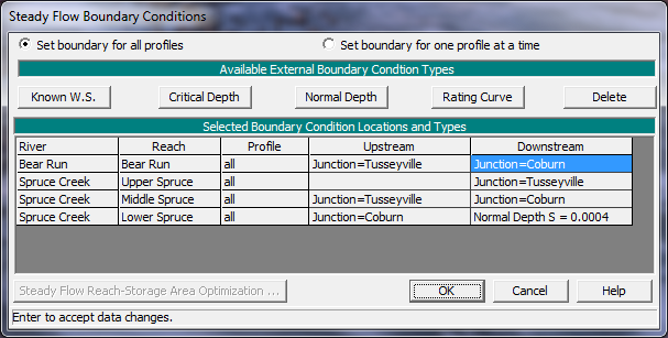
After the flow data were entered, the boundary conditions were established. This was performed by selecting the Boundary Conditions icon from the top of the Steady Flow Data Editor. This resulted in the display as shown in the figure below. As shown, the boundary conditions table will automatically contain any internal boundary conditions such as stream junctions. The user is required to enter the external boundary conditions. For this example, a subcritical flow analysis was performed; therefore, the external boundary condition at the downstream end of Lower Spruce was specified. Normal Depth was chosen with a slope of 0.0004 ft/ft. After the boundary condition was entered, the editor was closed and the flow data was saved as "10, 50, and 100 year flow events."

Steady Flow Data Analysis

After the geometric and flow data were entered, the files were then saved as a plan. This was performed by selecting Run and then Steady Flow Analysis from the main program window. This activated the Steady Flow Analysis Window as shown in the figure below. In the steady flow window, first the Short ID of "Loop" was entered. Next, the geometry file "Looped Geometry" and the steady flow data file "10, 50, and 100 year flow events" were selected by depressing the down arrows on the right side of the window.

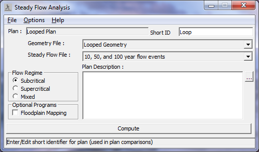
(Note: Since there was only 1 geometry file and only 1 flow file, this was not necessary.) Then, File and Save Plan As were selected and the title "Looped Plan" was entered. The OK button was selected and the plan title appeared near the top of the steady flow window. Finally, the Flow Regime was selected as subcritical and the COMPUTE button was selected.

Analysis of Results for Initial Flow Distribution

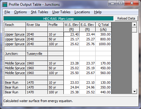
The user can review the results of the analysis both graphically and in tabular format. For this example, this discussion will initially be concerned with the flow distribution as selected for Bear Run and Middle Spruce. To determine the adequacy of the previously chosen flow distribution, the energy gradeline elevations at the upstream end of Bear Run and Middle Spruce will be compared. To determine the calculated energy values, the Junction Table was reviewed and a portion of the table is shown in the figure below. This table was activated from the main program window by selecting View, Profile Summary Table, Std. Tables, and then JunctionTable 1.

The rows in the table in the figure below are divided into groups of three, one row for each of the three profiles. The first column of the table displays the river reach, the second column displays the river station, and the third column lists the water surface elevation for the particular river station. As can be seen in the figure below, for the river reach of Middle Spruce at the river station 1960 (the upstream station), the flow rates were 170, 450, and 560 cfs, and the energy gradeline elevations were 23.37, 25.19, and 25.67 feet for the three flow profiles. The energy gradeline elevations for the upstream river station of Bear Run (river station 1470) were 23.10, 24.96, and 25.52 feet. By comparing these values, it can be seen that the energy gradelines differ by 0.27, 0.23, and 0.15 feet for the three profiles, respectively.

Since the upstream river stations on Middle Spruce and Bear Run were located close to the stream junction, the energy gradeline elevations for these two river stations should be approximately equal. Therefore, the flow rates for Middle Spruce and Bear Run were redistributed and a subsequent analysis was performed. This is discussed in the next section.

Steady Flow Analysis with New Flow Distribution

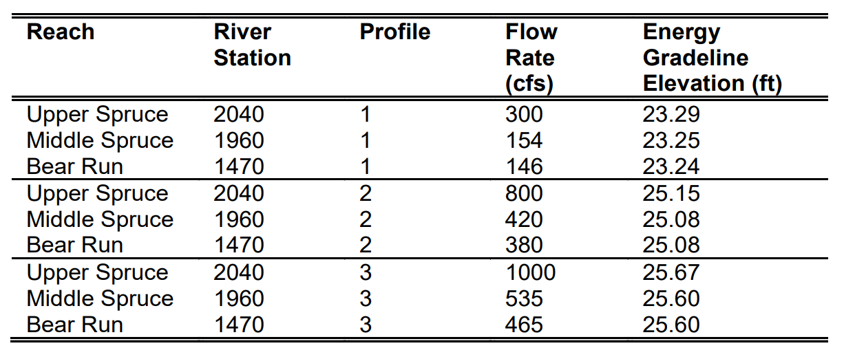
After reviewing the energy gradeline values at the upstream river stations for Middle Spruce and Bear Run, the flow rates for these river reaches were redistributed. Since the energy values for Bear Run were lower than that of Middle Spruce for all three of the profiles, a greater portion of the total flow was apportioned to Bear Run for all of the profiles. To perform this, the Steady Flow Data Editor was activated and the flow values were adjusted. Then a subsequent analysis was performed and the energy values compared. This procedure was continued until the energy values were within a reasonable tolerance. The table below shows the final flow distribution and the resulting energy gradeline values for the upstream river stations of Middle Spruce and Bear Run.

Additionally, the table shows the energy gradeline values for the downstream river station of Upper Spruce Creek. These values should be greater than the energy values for the upstream river stations of Middle Spruce and Bear Run. The final energy values for Middle Spruce and Bear Run are within a reasonable tolerance for each profile. Therefore, the flow distribution as shown in Table 8.1 was considered as a reasonable estimate of the flow rates through each river reach.

Analysis of Results for Final Flow Distribution

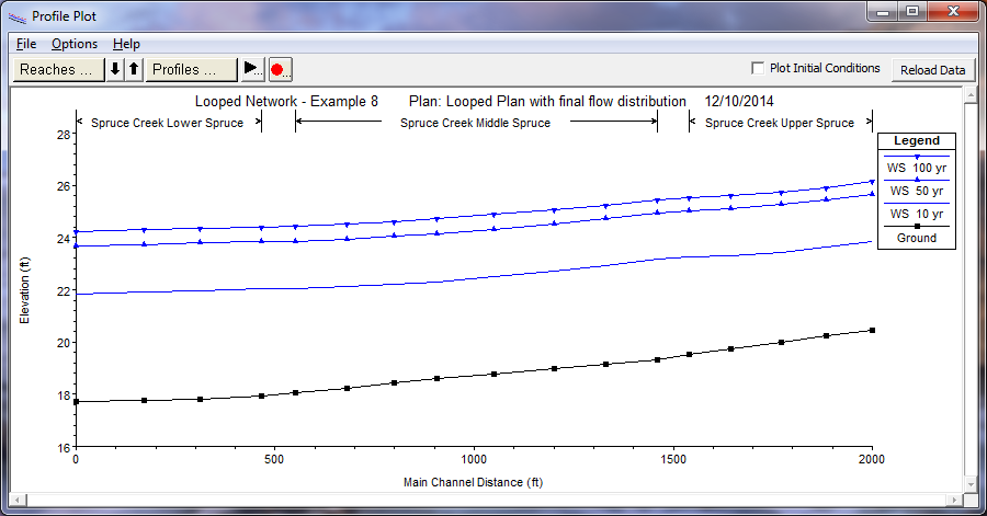
For an additional review of the flow distribution for the looped plan, the profile plot is shown in the figure below. To activate the profile plot, from the main program window select View and then Water Surface Profiles. For this plot, the reaches of Upper Spruce, Middle Spruce, and Lower Spruce Creek were selected. This represents the flow along the right side of the river schematic.

Similarly, the flow along the left edge of the river schematic can be viewed by selecting the river reach Bear Creek instead of Middle Spruce. This is performed by selecting Options, Reaches, and then the appropriate river reach.

Summary

As a summary for this example, a river system that contained a loop was analyzed. The flow rates for the branches of the loop were initially estimated and, after an initial analysis, the upstream energy values for each branch were compared. Since the initial energy values were not within a reasonable tolerance, the flow rates through each branch were redistributed and a subsequent analysis performed. This procedure was continued until the upstream energy values for the two branches were within a reasonable tolerance. By performing the flow distribution and energy comparison in this manner, it was necessary that the cross sections around the junction were spaced close together.